GuidingCenter · Particle orbits
Guiding-center orbits in a tokamak
Guiding centers with different pitch angles follow the field of a circular tokamak: particles with large parallel velocity circle the magnetic axis; others are reflected on the high-field side and bounce in banana-shaped orbits.
← All examples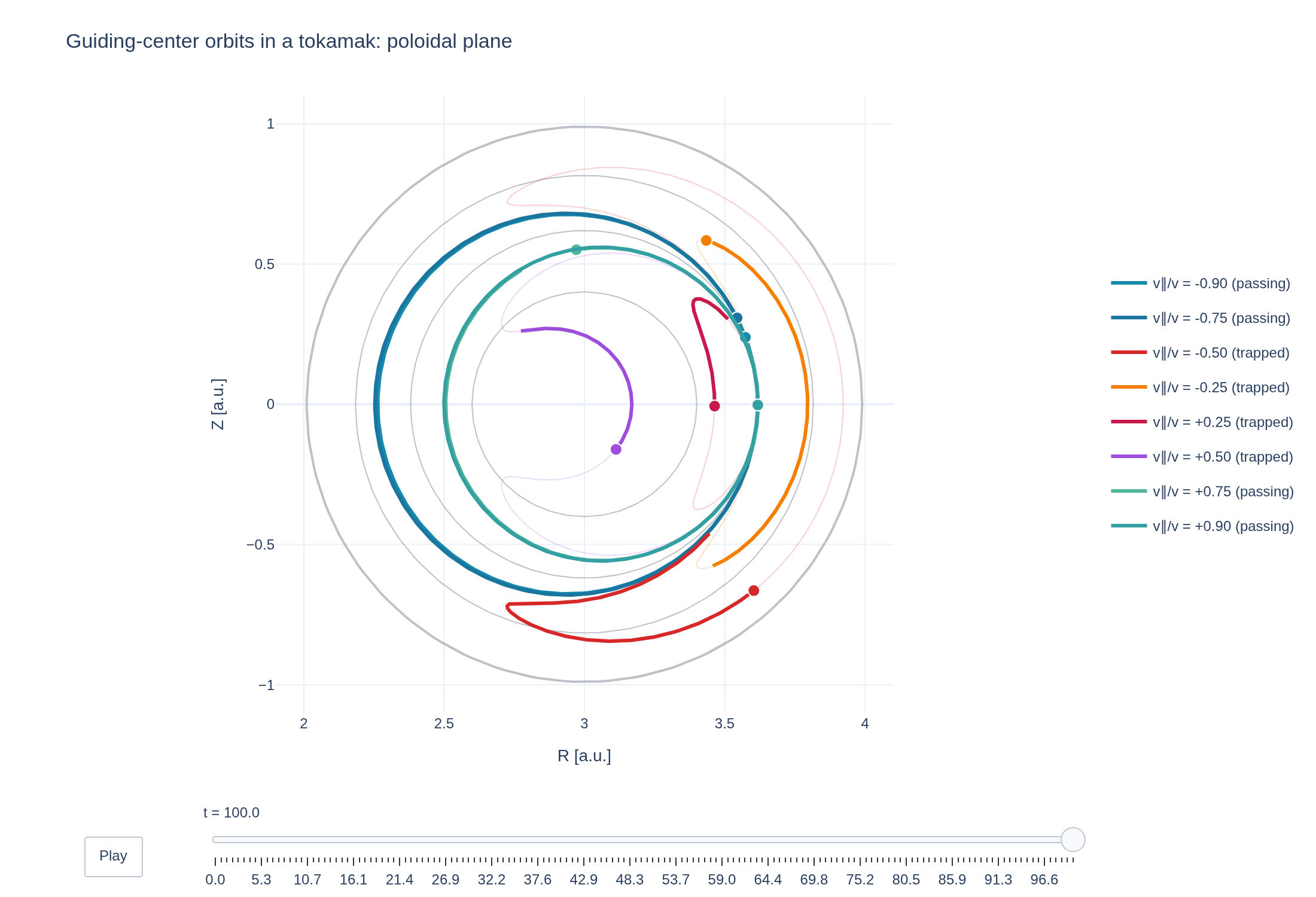


Physical problem
Passing and trapped guiding centers
The magnetic-field strength varies around a tokamak flux surface. At fixed energy and magnetic moment, an increase in field strength reduces the parallel kinetic energy. Particles with sufficiently small initial parallel speed reflect at mirror points and follow banana-shaped paths in the poloidal plane. Passing particles retain the sign of their parallel velocity and travel around the magnetic axis.
The example uses the analytic AdhocTorus equilibrium, projected onto spline spaces, and Strang splitting of the guiding-center propagators. All particles have initial speed 3; their initial parallel velocity fractions range from −0.9 to +0.9. The fixed-surface estimate of the trapping boundary is |v∥/v| ≈ 0.585. Finite orbit widths mean this estimate is not an exact classification rule; the labels below use observed parallel-velocity reversals.
The conservation diagnostic evaluates energy and canonical toroidal momentum particle by particle using the analytic equilibrium. It therefore includes the effect of approximating that equilibrium by splines as well as the time-integration error. It does not use the cached kinetic-energy scalar.
PDEs solved by model:
Guiding-center Vlasov equation:
where is the guiding center distribution and
- Model
- GuidingCenter
- Grid
- 32 × 64 × 1
- FEEC degree
- 3 × 3 × 1
- Integrator
- Discrete gradient 1st order
- Evolution
- 2,000 steps
- Visualization
- Plotly
Performance
Profiling
Struphy's built-in scope-profiler instruments every propagator, pusher and solver call — these are the real per-call timings from the run above, rendered live from its data.
Gantt (rank 0)
Region statistics
| Region | Count | Avg (s) | Min (s) | Max (s) | Total (s) |
|---|
Complete source
Run the simulation
Requires the Struphy revision pinned by this site, with compiled kernels, Plotly and Kaleido. Run struphy compile once, then execute python guiding-center-orbits.py.
"""Guiding-center orbits in a tokamak: passing and trapped particles.

Eight guiding centers start on the outboard midplane of one flux surface with the same energy and
different pitch v_parallel / v. In the field of a circular tokamak the field strength is larger on
the inner side, so particles with a small parallel velocity are reflected there and bounce back and
forth (trapped, banana-shaped orbits in the poloidal plane), while faster particles circle the
magnetic axis (passing). The static magnetic field does no work, so the energy and the canonical
toroidal momentum of every particle are conserved, which checks the guiding-center pusher.

Adapted from Struphy's particle-tracing tutorial (tutorials/tutorial_particle_tracing.ipynb).

Requires Struphy 3.2 with compiled kernels (`struphy compile`).
"""

import numpy as np
import plotly.graph_objects as go
from plotly.subplots import make_subplots

from struphy import (
    BoundaryParameters,
    DerhamOptions,
    EnvironmentOptions,
    LoadingParameters,
    SavingParameters,
    Simulation,
    Time,
    WeightsParameters,
    domains,
    equils,
    grids,
    maxwellians,
)
from struphy.models import GuidingCenter

# A circular tokamak (minor radius 1, major radius 3) with a field strength of 2 on the axis.
equil = equils.AdhocTorus(B0=2.0)
domain = domains.Tokamak(equilibrium=equil, num_elements=(4, 16), degree=(2, 3))
equil.domain = domain

# Eight markers on the outboard midplane of the flux surface eta1 = 0.5, all with speed 3 and
# different pitch. The state of a guiding center is (position, v_parallel, mu), with the magnetic
# moment mu = v_perp^2 / (2 B) chosen from the pitch at the starting point.
speed = 3.0
pitches = (-0.9, -0.75, -0.5, -0.25, 0.25, 0.5, 0.75, 0.9)
start_eta1 = 0.5
b_start = float(equil.absB0(start_eta1, 0.0, 0.0, squeeze_out=True))
initial = tuple(
    (start_eta1, 0.0, 0.0, speed * pitch, speed**2 * (1.0 - pitch**2) / (2.0 * b_start)) for pitch in pitches
)

model = GuidingCenter()
model.kinetic_ions.set_markers(
    loading_params=LoadingParameters(Np=len(initial), seed=1, specific_markers=initial),
    weights_params=WeightsParameters(),
    # A marker that leaves through the plasma edge is removed; the angles are periodic.
    boundary_params=BoundaryParameters(bc=("remove", "periodic", "periodic")),
    saving_params=SavingParameters(n_markers=1.0),
    bufsize=2.0,
)
model.propagators.push_bxe.options = model.propagators.push_bxe.Options(tol=1e-5)
model.propagators.push_parallel.options = model.propagators.push_parallel.Options(tol=1e-5)
model.kinetic_ions.var.add_background(maxwellians.GyroMaxwellian2D(n=(1.0, None), B0=b_start))

# The equilibrium is projected onto splines, which the guiding-center pusher evaluates.
grid = grids.TensorProductGrid(num_elements=(32, 64, 1))
derham_opts = DerhamOptions(degree=(3, 3, 1), bcs=(("free", "free"), None, None))

env = EnvironmentOptions(
    out_folders="struphy_gallery_runs",
    sim_folder="guiding_center_orbits",
)
sim = Simulation(
    model=model,
    name="Guiding-center orbits in a tokamak",
    description=(
        "Guiding centers with different pitch angles follow the field of a circular tokamak: "
        "particles with large parallel velocity circle the magnetic axis; others are reflected on the high-field "
        "side and bounce in banana-shaped orbits."
    ),
    env=env,
    time_opts=Time(dt=0.05, Tend=100.0, split_algo="Strang"),
    domain=domain,
    equil=equil,
    grid=grid,
    derham_opts=derham_opts,
)

if __name__ == "__main__":
    from _gallery import export_profiling, merge_metadata, publish_thumbnail, save_extra_figure, save_figure

    output = sim.run(profiling_activated=True)
    output.pproc()

    # (t, marker, quantity) with the quantities named x, y, z, v1, v2, ...: the position in Cartesian
    # coordinates, then the parallel velocity (v1) and the magnetic moment (v2) of a 5D marker. The
    # labels after v2 do not describe these columns and are not used here.
    orbits = output.evaluate("kinetic_ions")
    times = orbits.t.values
    x, y, z = (orbits.sel(quantity=name).values for name in ("x", "y", "z"))
    v_parallel = orbits.sel(quantity="v1").values
    moment = orbits.sel(quantity="v2").values
    major_radius = np.hypot(x, y)
    n_markers = x.shape[1]

    # Trapped particles are reflected: their parallel velocity changes sign along the orbit.
    reflections = (np.diff(np.sign(v_parallel), axis=0) != 0).sum(axis=0)
    trapped = reflections > 0
    labels = [f"v∥/v = {pitch:+.2f} ({'trapped' if trapped[i] else 'passing'})" for i, pitch in enumerate(pitches)]
    print("reflections per marker:", reflections.tolist())

    # The trapping boundary at the outboard midplane from the field strength on the starting surface:
    # a particle is trapped if v_parallel^2 < 2 mu (B_max - B_start).
    poloidal_angle = np.linspace(0.0, 1.0, 400, endpoint=False)
    surface_x, surface_y, surface_z = domain(start_eta1, poloidal_angle, 0.0, squeeze_out=True)
    surface_field = np.linalg.norm(
        np.array(equil.b_xyz(surface_x.ravel(), surface_y.ravel(), surface_z.ravel())), axis=0
    )
    boundary_pitch = float(np.sqrt(1.0 - b_start / surface_field.max()))
    print(f"Trapping boundary from the field on the starting surface: |v∥/v| = {boundary_pitch:.3f}")

    # Conserved quantities per marker: the energy v_par^2 / 2 + mu B, and the canonical toroidal momentum
    # R v_par b_phi - psi / epsilon (psi is set to zero on the magnetic axis). The magnetic moment is a
    # phase-space coordinate of the model and constant by construction.
    field = np.array(equil.b_xyz(x.ravel(), y.ravel(), z.ravel())).reshape(3, *x.shape)
    field_strength = np.linalg.norm(field, axis=0)
    toroidal_angle = np.arctan2(-y, x)
    toroidal_unit = np.array([-np.sin(toroidal_angle), -np.cos(toroidal_angle), np.zeros_like(x)])
    b_toroidal = (field * toroidal_unit).sum(axis=0) / field_strength
    epsilon = float(model.kinetic_ions.equation_params.epsilon)
    flux = equil.psi(major_radius, z) - float(equil.psi_range[0])
    energy = 0.5 * v_parallel**2 + moment * field_strength
    momentum = major_radius * v_parallel * b_toroidal - flux / epsilon
    energy_drift = np.abs(energy - energy[0]) / np.abs(energy[0])
    # P_phi can be nearly zero by cancellation. Normalize by the sum of the
    # magnitudes of its initial mechanical and flux contributions instead.
    momentum_scale = np.abs(major_radius[0] * v_parallel[0] * b_toroidal[0]) + np.abs(flux[0] / epsilon)
    momentum_drift = np.abs(momentum - momentum[0]) / momentum_scale
    print(f"Largest relative drift: energy {energy_drift.max():.2e}, canonical momentum {momentum_drift.max():.2e}")
    lost = int(output.scalars["n_lost_particles"].max())

    # The half period between two reflections is the time a trapped particle needs to go from one
    # mirror point to the other.
    half_periods = []
    for i in np.flatnonzero(reflections >= 2):
        crossings = times[1:][np.diff(np.sign(v_parallel[:, i])) != 0]
        half_periods.extend(np.diff(crossings))
    bounce_period = 2.0 * float(np.mean(half_periods))
    print(f"Bounce period of the trapped particles: {bounce_period:.1f}")

    trapped_colors = ["#d62828", "#f77f00", "#c9184a", "#9d4edd"]
    passing_colors = ["#168aad", "#1a759f", "#52b69a", "#34a0a4"]
    colors = []
    for i in range(n_markers):
        palette = trapped_colors if trapped[i] else passing_colors
        colors.append(palette[sum(1 for j in range(i) if trapped[j] == trapped[i]) % len(palette)])

    # The flux surfaces in the poloidal plane, for context.
    surfaces = np.array([0.25, 0.5, 0.75, 1.0])
    surface_x, surface_y, surface_z = domain(surfaces, np.linspace(0.0, 1.0, 200), 0.0, squeeze_out=True)
    surface_r = np.hypot(surface_x, surface_y)

    def add_flux_surfaces(figure, **position):
        for i in range(len(surfaces)):
            figure.add_trace(
                go.Scatter(
                    x=surface_r[i],
                    y=surface_z[i],
                    mode="lines",
                    line={"color": "rgba(110,120,130,0.45)", "width": 2 if surfaces[i] == 1.0 else 1},
                    hoverinfo="skip",
                    showlegend=False,
                ),
                **position,
            )

    # The animation: every guiding center is a bright head with a trail of its last 15 time units,
    # over its faint full path.
    tail = 300
    n_frames = 150
    picks = np.linspace(0, len(times) - 1, n_frames, dtype=int)
    figure = go.Figure()
    add_flux_surfaces(figure)
    for i in range(n_markers):
        figure.add_trace(
            go.Scatter(
                x=major_radius[:, i],
                y=z[:, i],
                mode="lines",
                line={"color": colors[i], "width": 1},
                opacity=0.2,
                hoverinfo="skip",
                showlegend=False,
                legendgroup=str(i),
            )
        )

    def moving_traces(index):
        traces = []
        for i in range(n_markers):
            start = max(0, index - tail)
            traces.append(
                go.Scatter(
                    x=major_radius[start : index + 1, i],
                    y=z[start : index + 1, i],
                    mode="lines",
                    line={"color": colors[i], "width": 3},
                    name=labels[i],
                    legendgroup=str(i),
                )
            )
            traces.append(
                go.Scatter(
                    x=[major_radius[index, i]],
                    y=[z[index, i]],
                    mode="markers",
                    marker={"color": colors[i], "size": 10, "line": {"color": "white", "width": 1}},
                    showlegend=False,
                    legendgroup=str(i),
                )
            )
        return traces

    first_moving = len(figure.data)
    for trace in moving_traces(0):
        figure.add_trace(trace)
    moving_indices = list(range(first_moving, len(figure.data)))
    frames = [go.Frame(name=f"{times[index]:.1f}", data=moving_traces(index), traces=moving_indices) for index in picks]
    figure.frames = frames
    figure.update_xaxes(range=[1.9, 4.1], title_text="R [a.u.]", constrain="domain")
    figure.update_yaxes(range=[-1.1, 1.1], title_text="Z [a.u.]", scaleanchor="x", scaleratio=1)
    figure.update_layout(
        title="Guiding-center orbits in a tokamak: poloidal plane",
        template="plotly_white",
        autosize=True,
        margin={"l": 70, "r": 30, "t": 80, "b": 130},
        legend={"x": 1.02, "y": 0.5, "yanchor": "middle"},
        updatemenus=[
            {
                "type": "buttons",
                "showactive": False,
                "x": 0.0,
                "xanchor": "left",
                "y": -0.2,
                "yanchor": "top",
                "buttons": [
                    {
                        "label": "Play",
                        "method": "animate",
                        "args": [None, {"frame": {"duration": 40, "redraw": True}, "fromcurrent": True}],
                    },
                ],
            },
        ],
        sliders=[
            {
                "steps": [
                    {
                        "args": [[frame.name], {"frame": {"duration": 0, "redraw": True}, "mode": "immediate"}],
                        "label": frame.name,
                        "method": "animate",
                    }
                    for frame in frames
                ],
                "active": 0,
                "x": 0.12,
                "len": 0.88,
                "y": -0.1,
                "currentvalue": {"prefix": "t = "},
            },
        ],
    )

    # The still image shows the end of the run, with all trails.
    still_traces = list(figure.data[:first_moving]) + moving_traces(len(times) - 1)
    save_figure(
        figure,
        "guiding-center-orbits",
        height=750,
        static_data=still_traces,
        static_active=len(frames) - 1,
    )

    # One panel per particle: the orbit in the poloidal plane.
    panels = make_subplots(rows=2, cols=4, subplot_titles=labels, horizontal_spacing=0.03, vertical_spacing=0.12)
    for i in range(n_markers):
        row, col = divmod(i, 4)
        add_flux_surfaces(panels, row=row + 1, col=col + 1)
        panels.add_trace(
            go.Scatter(
                x=major_radius[:, i],
                y=z[:, i],
                mode="lines",
                line={"color": colors[i], "width": 2.5},
                showlegend=False,
            ),
            row=row + 1,
            col=col + 1,
        )
        panels.add_trace(
            go.Scatter(
                x=[major_radius[0, i]],
                y=[z[0, i]],
                mode="markers",
                marker={"color": "#222", "size": 7, "symbol": "circle-open", "line": {"width": 2}},
                showlegend=False,
            ),
            row=row + 1,
            col=col + 1,
        )
        axis = i + 1
        panels.update_xaxes(range=[1.9, 4.1], showticklabels=row == 1, row=row + 1, col=col + 1)
        panels.update_yaxes(
            range=[-1.1, 1.1],
            showticklabels=col == 0,
            scaleanchor="x" if axis == 1 else f"x{axis}",
            scaleratio=1,
            row=row + 1,
            col=col + 1,
        )
    panels.update_xaxes(title_text="R [a.u.]", row=2)
    panels.update_yaxes(title_text="Z [a.u.]", col=1)
    panels.update_layout(
        title="Guiding-center orbits: one panel per particle (circle: start)",
        template="plotly_white",
        autosize=True,
        margin={"l": 70, "r": 30, "t": 100, "b": 60},
    )
    panels.update_annotations(font_size=12)

    # The parallel velocity over time: it changes sign for trapped particles.
    velocity = go.Figure()
    for i in range(n_markers):
        velocity.add_scatter(
            x=times,
            y=v_parallel[:, i] / speed,
            mode="lines",
            name=labels[i],
            line={"color": colors[i], "width": 2.5, "dash": "solid" if trapped[i] else "dot"},
        )
    velocity.add_hline(y=0.0, line={"color": "#888", "width": 1})
    velocity.update_layout(
        title="Parallel velocity of the guiding centers",
        xaxis_title="t [a.u.]",
        yaxis_title="v∥ / v",
        template="plotly_white",
        autosize=True,
        margin={"l": 70, "r": 30, "t": 80, "b": 60},
    )

    # The drift of the conserved quantities, on a logarithmic axis.
    floor = 1e-12
    conservation = make_subplots(rows=1, cols=2, subplot_titles=("Energy", "Canonical toroidal momentum"))
    for i in range(n_markers):
        for column, drift in enumerate((energy_drift, momentum_drift), start=1):
            conservation.add_scatter(
                x=times,
                y=np.maximum(drift[:, i], floor),
                mode="lines",
                name=labels[i],
                showlegend=column == 1,
                legendgroup=str(i),
                line={"color": colors[i], "width": 2, "dash": "solid" if trapped[i] else "dot"},
                row=1,
                col=column,
            )
    conservation.update_yaxes(type="log", title_text="relative change", col=1)
    conservation.update_yaxes(type="log", col=2)
    conservation.update_yaxes(exponentformat="power")
    conservation.update_xaxes(title_text="t [a.u.]")
    conservation.update_layout(
        title="Conserved quantities along the orbits",
        template="plotly_white",
        autosize=True,
        margin={"l": 70, "r": 30, "t": 100, "b": 60},
    )

    figures = [
        save_extra_figure(
            panels,
            "guiding-center-orbits",
            "panels",
            alt="Poloidal-plane orbits of eight guiding centers, one panel each",
            caption='The eight orbits start at the same position and speed, with different parallel velocity fractions. Four reflect and form banana-shaped paths; four pass around the magnetic axis. Grey curves mark flux surfaces and the open circle marks the initial position.',
        ),
        save_extra_figure(
            velocity,
            "guiding-center-orbits",
            "velocity",
            alt="Parallel velocity of the guiding centers against time",
            caption='The parallel velocity changes sign at each mirror reflection for trapped particles (solid curves). Passing particles (dotted curves) retain their initial sign. The normalization uses the common initial speed, not the instantaneous parallel speed.',
        ),
        save_extra_figure(
            conservation,
            "guiding-center-orbits",
            "conservation",
            alt="Relative change of energy and canonical toroidal momentum against time",
            caption='Changes in energy and canonical toroidal momentum evaluated using the analytic equilibrium along the computed orbits. Energy is normalized to its initial value. Momentum is normalized to the sum of the magnitudes of its initial mechanical and magnetic-flux contributions, since their sum can nearly cancel. Values below 1e-12 are clipped for the logarithmic display. These diagnostics include equilibrium projection and time-integration errors.',
        ),
    ]

    profiling = export_profiling(sim, "guiding-center-orbits")

    merge_metadata(
        "guiding-center-orbits",
        markers=n_markers,
        nTrapped=int(trapped.sum()),
        nPassing=int((~trapped).sum()),
        boundaryPitch=boundary_pitch,
        bouncePeriod=bounce_period,
        maxEnergyDrift=float(energy_drift.max()),
        maxMomentumDrift=float(momentum_drift.max()),
        lostMarkers=lost,
        speed=speed,
        equilibrium="AdhocTorus (a = 1, R0 = 3, B0 = 2)",
        figures=figures,
        **publish_thumbnail("guiding-center-orbits"),
        **profiling,
    )
Adapted from Struphy’s particle-tracing tutorial.