Fluid model
LinearMHD
Linear ideal MHD with zero-flow equilibrium for magnetohydrodynamic wave propagation.
Overview
equilibrium magnetic field and zero background flow. The model solves the linearized ideal magnetohydrodynamic equations, which couple fluid dynamics (density, velocity, pressure) with magnetic field evolution.
The linear MHD system supports three wave families:
- Alfvén waves: incompressible shear waves propagating along
- Fast magnetosonic waves: compressible waves with phase velocity above the Alfvén speed
- Slow magnetosonic waves: compressible waves with phase velocity below the Alfvén speed
All evolved quantities are perturbations around a stationary equilibrium:
- - density perturbation
- - velocity perturbation
- - pressure perturbation
- - magnetic field perturbation
The corresponding equilibrium quantities are:
- - background density
- - background pressure
- - background magnetic field
Use cases
including Alfvén and magnetosonic dynamics around a prescribed equilibrium.
Typical use cases include:
- verification of linear MHD wave dispersion and mode structure
- perturbative studies around static equilibria
- benchmark problems for ideal-MHD field-fluid coupling
Governing equations
PDEs solved by model:
Continuity (mass conservation):
Momentum (Lorentz force):
Energy (adiabatic process):
Induction (Faraday's law):
Normalization
The model therefore uses the Alfvén velocity as its characteristic speed scale.
Discretization
Diagnostics
The following scalars are tracked during simulation:
- Kinetic energy (perturbation):
- Magnetic energy (perturbation):
- Mean pressure perturbation: (
en_p). This is a linear diagnostic, not an energy. - Thermal perturbation energy: (
en_thermal), with - Total perturbed energy: (
en_tot) - Equilibrium magnetic energy:
- Equilibrium internal energy:
- Total magnetic energy:
Examples
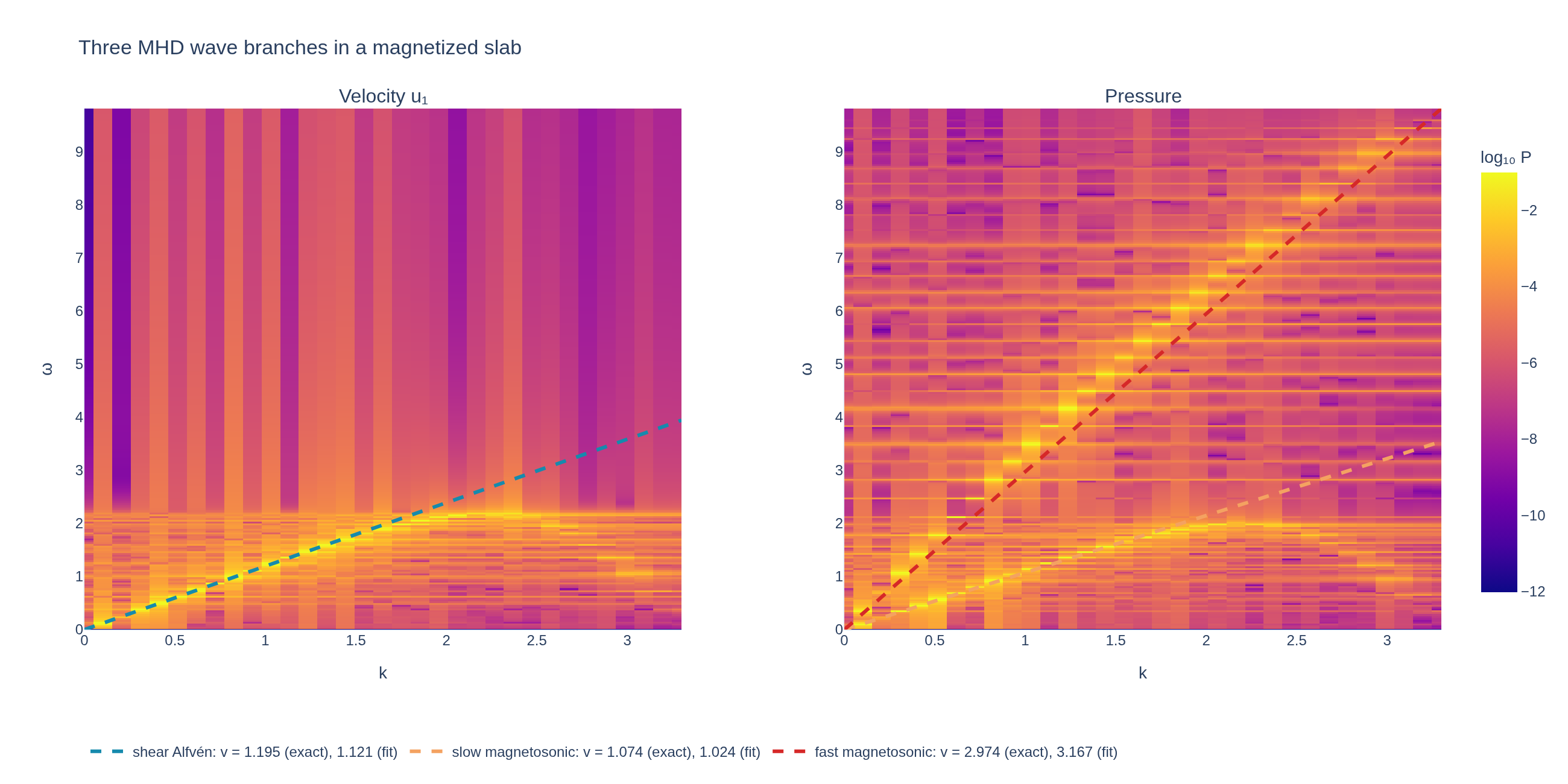
MHD waves in a magnetized slab
Broadband noise excites the shear Alfvén wave and the slow and fast magnetosonic waves of a uniform, obliquely magnetized plasma. The power spectra of the velocity and the pressure show the three branches, and their fitted speeds are compared with the exact ideal-MHD values. The equilibrium parameters are with and . All three velocity components receive coefficient noise of amplitude in a periodic interval .
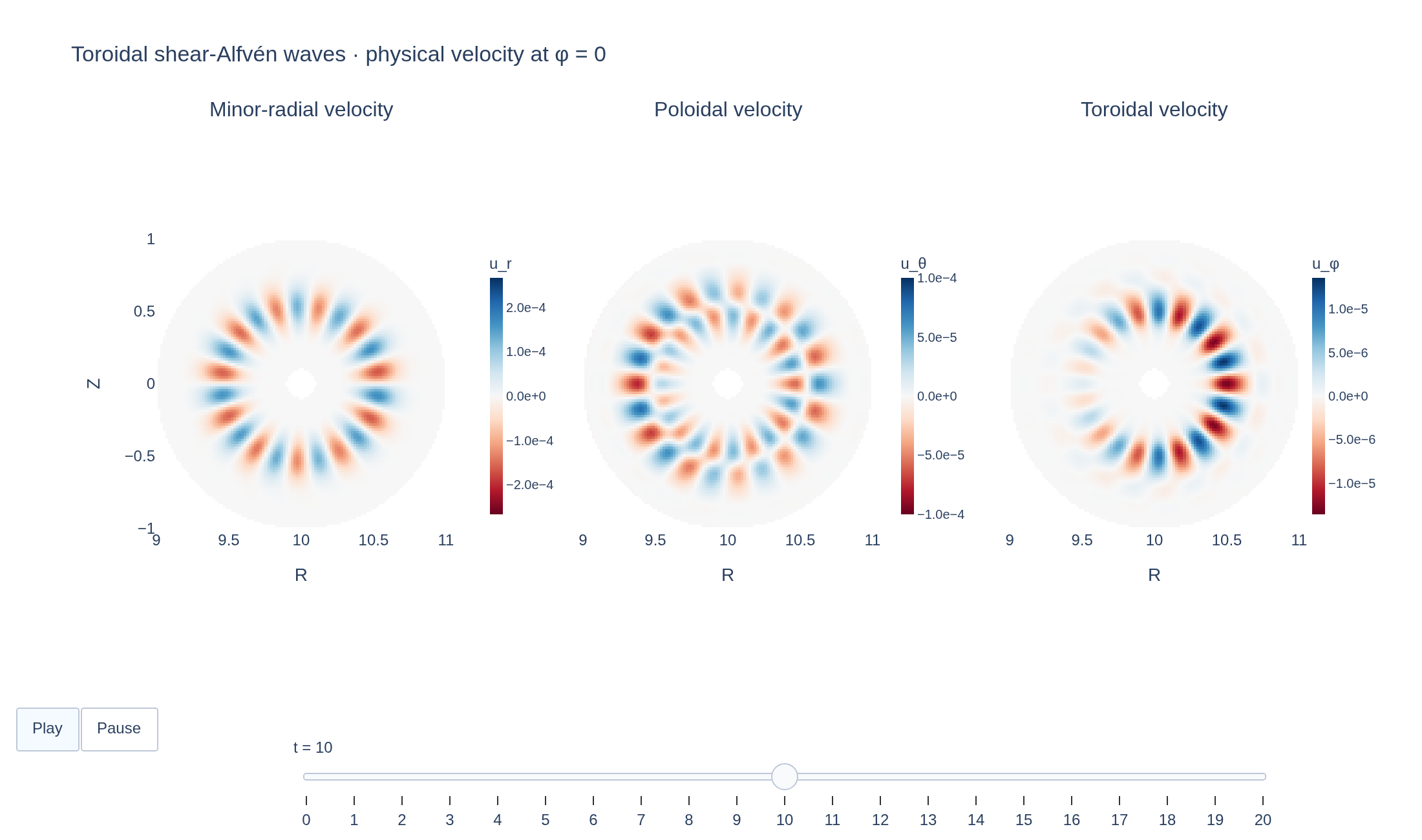
Toroidal shear-Alfvén waves
A local preview of coupled poloidal shear-Alfvén perturbations in a circular tokamak, evolved with LinearMHD, including its magnetosonic propagator. The hollow torus has , major radius , and a periodic one-sixth toroidal sector. The AdhocTorus equilibrium uses , , and . The initial logical velocity combines , sector modes with amplitude parameter and Gaussian profiles centered at with width ; the poloidal component uses their radial derivatives. The coarse grid and short duration are intended for exploration, not a converged TAE benchmark. Plots show physical minor-radial, poloidal and toroidal velocity on the φ=0 slice; each component keeps its own fixed color range throughout the animation.