Kinetic model

VlasovAmpereOneSpecies

Vlasov-Ampère system for a single kinetic species in an electric field.

Overview

This model couples the kinetic Vlasov equation for the particle distribution function

with Ampère's law for the electric field evolution. It includes the effect of a static background magnetic field $B_{0}$ and solves the initial Poisson equation to satisfy Gauss's law at $t = 0$ . The model uses a particle-in-cell (PIC) method with finite element exterior calculus (FEEC) for the electromagnetic fields.

All field variables are perturbations around a reference equilibrium distribution. The model enables studies of kinetic instabilities, particle-wave interactions, and nonlinear plasma physics without assuming a fluid approximation.

Use cases

This model is appropriate for:

studying kinetic instabilities in collisionless plasmas
particle-wave interactions and nonlinear plasma physics
initial value problems with prescribed equilibrium distributions
benchmark problems for kinetic-field coupling schemes
verification of PIC methods in simplified geometries

Governing equations

PDEs solved by model:

Vlasov equation:

\frac{\partial f}{\partial t} + v \cdot \nabla f + \frac{1}{ε} (E + v \times B_{0}) \cdot \frac{\partial f}{\partial v} = 0

Ampère's law:

- \frac{\partial E}{\partial t} = \frac{α ^{2}}{ε} \int_{R^{3}} v f d^{3} v

Initial Poisson equation: At $t = 0$ , solve weakly for the electric potential $ϕ$ :

\int_{Ω} \nabla ψ^{⊤} \cdot \nabla ϕ d x = \frac{α ^{2}}{ε} \int_{Ω} \int_{R^{3}} ψ (f - f_{0}) d^{3} v d x \forall ψ \in H^{1} E (t = 0) = - \nabla ϕ (t = 0)

Normalization

Velocity and field normalizations:

v^= c, E^= B^v^, ϕ^= E^x^

Dimensionless parameters:

α = \frac{ω ^ _{p}}{ω ^ _{c}}, ε = \frac{1}{ω ^ _{c} t ^}

where

ω^_{p} = \frac{n ^ ( Z e ) ^{2}}{ϵ _{0} ( A m _{H} )}, ω^_{c} = \frac{( Z e ) B ^}{( A m _{H} )}

For electrons: $Z = - 1$ , $A = 1/1836$ .

Discretization

Time integration is performed by the following propagators (in sequence):

PushEta
PushVxB (if with_B0 is True)
VlasovAmpereCoupling

Diagnostics

The following scalars are tracked during simulation:

Electric field energy: $E_{E} = \frac{1}{2} \int ∣ E ∣^{2} d V$
Kinetic energy: $E_{f} = \frac{α ^{2}}{2 N} \sum_{p} w_{p} ∣ v_{p} ∣^{2}$
Total energy: $E_{tot} = E_{E} + E_{f}$

Examples

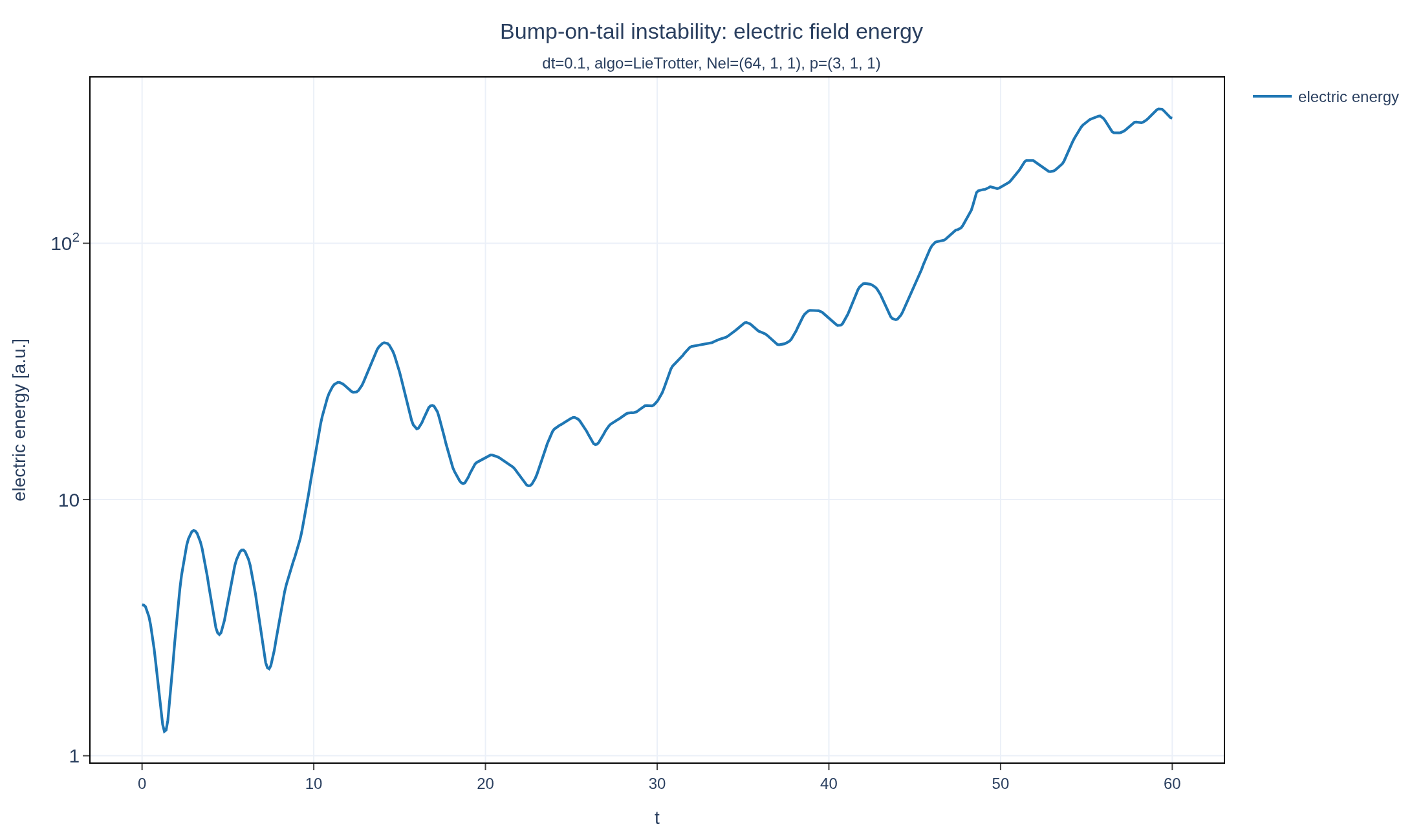
Bump-on-tail instability

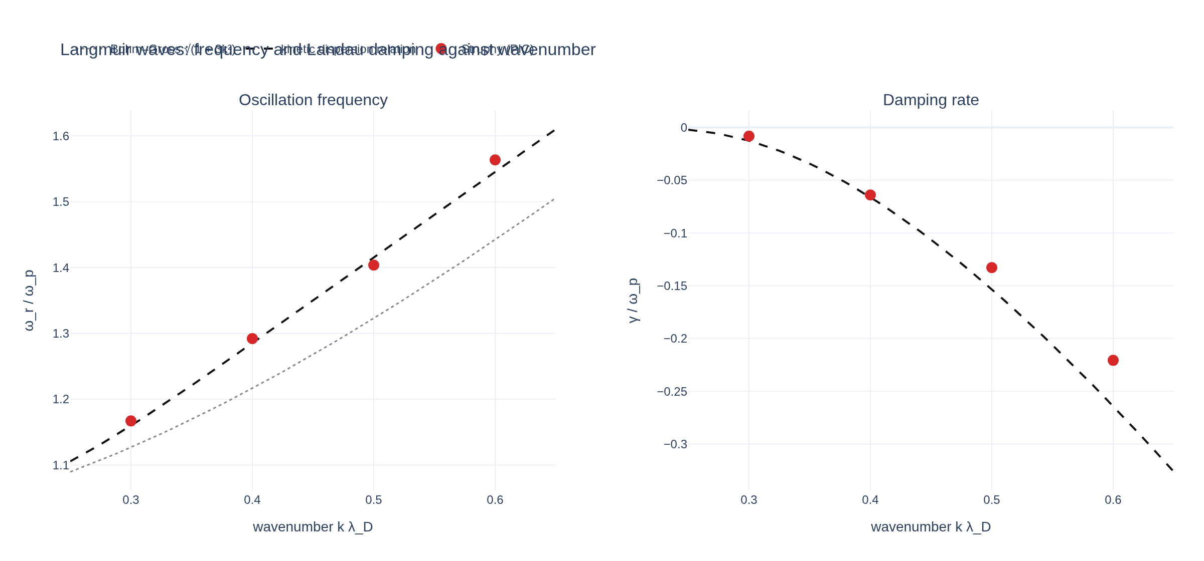
A minority “bump” of fast particles on the tail of an otherwise Maxwellian distribution drives Langmuir waves unstable, feeding energy into the field until particle trapping saturates it. The bulk has $n_b=0.9$ , $u_{x,b}=3$ and $v_{\mathrm{th},x,b}=1$ . Only the fast population is perturbed: $n_h(x,0)=0.1+0.05\cos(2\pi x/L),\qquad u_{x,h}=-4.5,\qquad v_{\mathrm{th},x,h}=0.5,$ with $L=62.83$ .

Langmuir wave dispersion

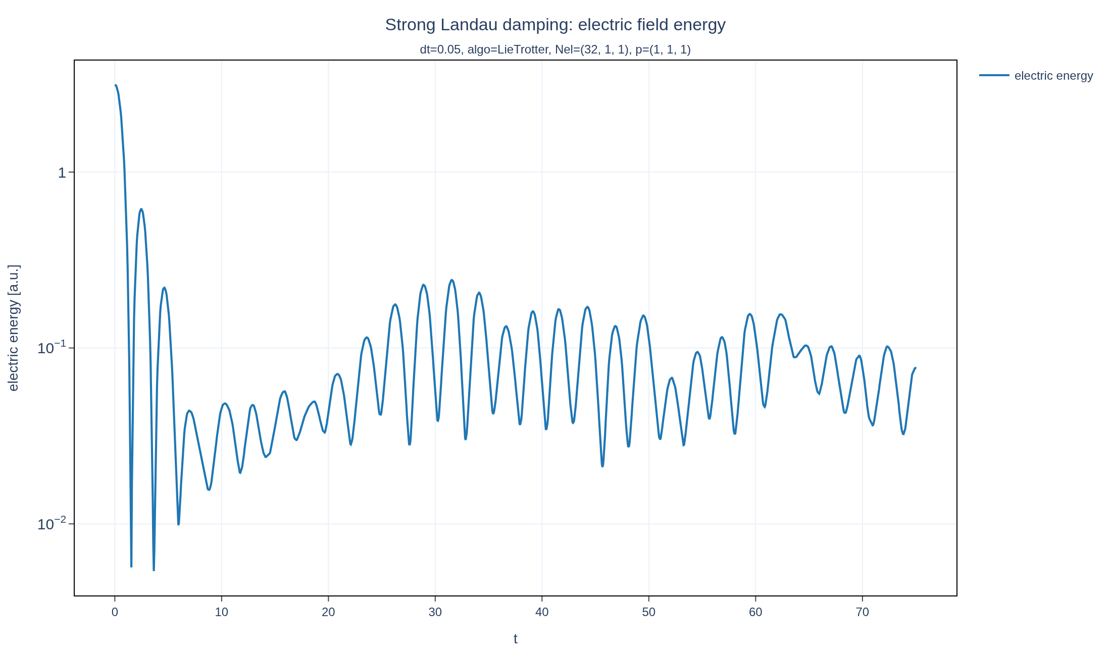
A density perturbation in a uniform Maxwellian plasma oscillates as a Langmuir wave and is Landau damped. Runs at four wavenumbers give the oscillation frequency and the damping rate against k, and are compared with the root of the kinetic dispersion relation and with the fluid Bohm–Gross estimate. Each run starts from a zero-drift, unit-thermal-speed Maxwellian with $n(x,0)=1+10^{-3}\cos(kx),\qquad L_x=2\pi/k,$ for $k\in\{0.3,0.4,0.5,0.6\}$ .

Strong Landau damping

A large-amplitude perturbation drives a Vlasov-Ampère plasma into the nonlinear regime — particles trap in the field's potential wells, and the field energy bounces instead of decaying smoothly. The initial Maxwellian has density $n(x,0)=1+0.5\cos(2\pi x/L),\qquad L=12.56,$ zero mean velocity and thermal speed $v_{\mathrm{th}}=1$ .

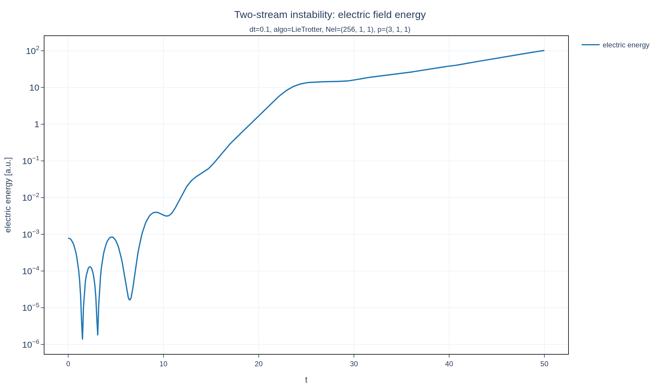
Two-stream instability

Two counter-streaming Maxwellian beams are kinetically unstable — a tiny perturbation grows exponentially, drawing energy from the beams, until particle trapping saturates the growth. The two beams start with $n_\pm(x,0)=0.5+10^{-3}\cos(2\pi x/L),\qquad u_{x,\pm}=\pm3,$ where $L=31.42$ and each beam has thermal speed $v_{\mathrm{th}}=1$ .

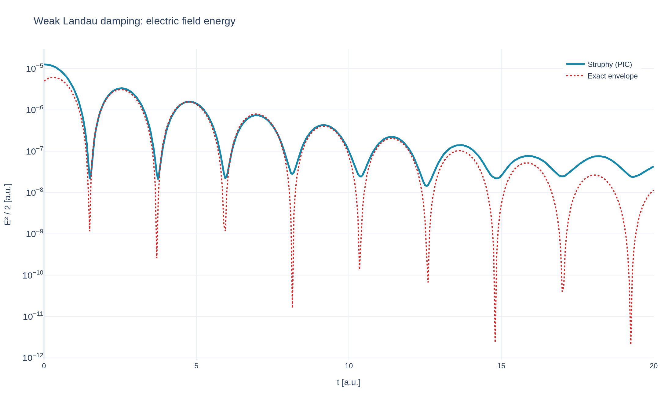
Weak Landau damping

A tiny electrostatic perturbation phase-mixes away in a collisionless plasma — the classic Landau-damping benchmark, compared here against the linear damping rate $\gamma \approx -0.1533$ at wavenumber $k \approx 0.5$ in normalized units. The initial Maxwellian has density $n(x,0)=1+10^{-3}\cos(2\pi x/L),\qquad L=12.56,$ zero mean velocity and thermal speed $v_{\mathrm{th}}=1$ .