
Quickstart#
Struphy is a Python API for solving PDEs with structure-preserving discretizations. This quickstart shows how to solve a simple problem with minimal input: a 1D Poisson solve.
For interactive tutorials (no local install), use mybinder. For more examples, see Userguide and the tutorial collection.
Solve Poisson In A Few Steps#
Make sure that Struphy is installed and compiled (see Install and compile).
Save the code below as params_poisson.py. By default, output is written to
sim_1/ in the directory from which you launch the script (change this with
EnvironmentOptions).
We search for a potential \(\phi(x, y)\) satisfying the Poisson equation
for a given source term \(\rho(x)\) on a doubly periodic 2D domain.
Import the API and choose a model.
import numpy as np
from matplotlib import pyplot as plt

from struphy import Simulation, domains, grids, perturbations
from struphy.models import Poisson
Create the
Poissonmodel.
model = Poisson()
3. This model features the Propagator PoissonSolve under propagators.poisson.
For periodic boundary conditions we will stabilize via options.
stab_eps = 1e-8

model.propagators.poisson.options = model.propagators.poisson.Options(
    stab_eps=stab_eps,
)
Add a manufactured term \(\rho(x) = (k^2 + \epsilon)\cos(kx)\) to the
sourcevariable.
Lx = 2.0 * np.pi
Ly = 4.0 * np.pi
mode = 2
k = mode * 2.0 * np.pi / Lx
source_amp = k**2 + stab_eps

fun = perturbations.ModesCos(ls=(mode,), amps=(source_amp,))

model.em_fields.source.add_perturbation(fun)
Build domain and grid, then instantiate a simulation.
domain = domains.Cuboid(r1=Lx, l2=-Ly / 2, r2=Ly / 2)
grid = grids.TensorProductGrid(num_elements=(64, 64, 1))

sim = Simulation(model=model, domain=domain, grid=grid)
Run the simulation.
sim.run()returns anOutputobject, the entry point for all post-processing.
out = sim.run()
Evaluate the potential on a line along \(\eta_1\) and compare to the exact solution.
out.evaluate()takes a"species/variable"name, evaluates the saved spline field on the given logical coordinates, and returns a labeledxarray.DataArray. Scalars fix a direction (here \(\eta_2 = \eta_3 = 0.5\)); omitted directions stay on the cell centres of the simulation grid.t=-1selects the last saved snapshot. The array also carries the physical coordinatesX, Y, Zso that xarray’s.plot()can use either coordinate system.
fig, axs = plt.subplots(1, 2, figsize=(12, 4))

eta1 = np.linspace(0, 1, 100)
phi_1d = out.evaluate("em_fields/phi", eta1=eta1, eta2=0.5, eta3=0.5, t=-1)

x = phi_1d["X"]
phi_exact = np.cos(k * x)
phi_exact_logical = np.cos(Lx * k * eta1)

phi_1d.plot(ax=axs[0], label="Struphy")  # plot along eta1 (default)
phi_1d.plot(ax=axs[1], x="X", label="Struphy")  # plot along physical X
axs[0].plot(eta1, phi_exact_logical, "k--", lw=1.8, label="exact")
axs[1].plot(x, phi_exact, "k--", lw=1.8, label="exact")

for ax in axs:
    ax.legend()
    ax.grid(alpha=0.3)
fig.savefig("quickstart_poisson_phi.png", dpi=150)
plt.show()
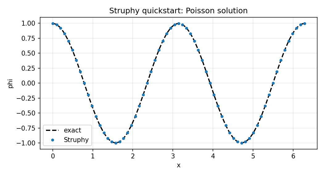
Exact (dashed) and Struphy solutions from Step 7, along \(\eta_1\) (left) and \(x\) (right).#
Evaluate on a 2D logical grid and plot in physical coordinates.
eta = np.linspace(0, 1, 100)
phi_2d = out.evaluate("em_fields/phi", eta1=eta, eta2=eta, t=-1)
phi_2d.plot(x="X", y="Y")
plt.show()
out can also be created later from the output folder alone, e.g. in a separate
post-processing script, via out = Output("sim_1"); the model, domain and numerical
options are reconstructed from run_metadata.json.
Full script (save as params_poisson.py and run with python params_poisson.py):
import numpy as np
from matplotlib import pyplot as plt

from struphy import Simulation, domains, grids, perturbations
from struphy.models import Poisson

model = Poisson()

stab_eps = 1e-8

model.propagators.poisson.options = model.propagators.poisson.Options(
    stab_eps=stab_eps,
)

Lx = 2.0 * np.pi
Ly = 4.0 * np.pi
mode = 2
k = mode * 2.0 * np.pi / Lx
source_amp = k**2 + stab_eps

fun = perturbations.ModesCos(ls=(mode,), amps=(source_amp,))

model.em_fields.source.add_perturbation(fun)

domain = domains.Cuboid(r1=Lx, l2=-Ly / 2, r2=Ly / 2)
grid = grids.TensorProductGrid(num_elements=(64, 64, 1))

sim = Simulation(model=model, domain=domain, grid=grid)

if __name__ == "__main__":
    # sim.run() returns an Output object for post-processing
    out = sim.run()

    # out.evaluate() evaluates a saved field on logical coordinates (eta1, eta2, eta3)
    # and returns a labeled xarray.DataArray; scalar etas fix a direction, omitted etas stay
    # on the simulation grid's cell centres, t=-1 selects the last snapshot. Physical coordinates X, Y, Z are attached.
    fig, axs = plt.subplots(1, 2, figsize=(12, 4))

    eta1 = np.linspace(0, 1, 100)
    phi_1d = out.evaluate("em_fields/phi", eta1=eta1, eta2=0.5, eta3=0.5, t=-1)

    x = phi_1d["X"]
    phi_exact = np.cos(k * x)
    phi_exact_logical = np.cos(Lx * k * eta1)

    # xarray plotting: along eta1 by default, or along any attached coordinate
    phi_1d.plot(ax=axs[0], label="Struphy")
    phi_1d.plot(x="X", ax=axs[1], label="Struphy")
    axs[0].plot(eta1, phi_exact_logical, "k--", lw=1.8, label="exact")
    axs[1].plot(x, phi_exact, "k--", lw=1.8, label="exact")

    for ax in axs:
        ax.legend()
        ax.grid(alpha=0.3)
    fig.savefig("quickstart_poisson_phi.png", dpi=150)
    plt.show()

    # 2D evaluation on a logical tensor-product grid, plotted in physical coordinates
    eta = np.linspace(0, 1, 100)
    phi_2d = out.evaluate("em_fields/phi", eta1=eta, eta2=eta, t=-1)
    phi_2d.plot(x="X", y="Y")
    plt.show()
Same Workflow For All Models#
The same Simulation API is reused across models. For example, replace Poisson with Maxwell:
from pathlib import Path

from struphy import EnvironmentOptions, Simulation, perturbations
from struphy.models import Maxwell

model = Maxwell()
model.em_fields.e_field.add_perturbation(
    perturbations.ModesCos(ls=(1,), amps=(1e-2,), comp=1)
)

env = EnvironmentOptions(sim_folder="sim_data")
sim = Simulation(model=model, env=env, params_path=__file__)
if __name__ == "__main__":
    sim.run()
Check Models for more models and their specific options.
Generate A Default Parameter File#
You can generate a ready-to-edit parameter file for any model from the CLI:
struphy params Poisson
This writes params_Poisson.py in your current directory. You can open and edit it, then run with:
python params_Poisson.py
As all data structures in Struphy are written for MPI, you can run the same script with mpirun to use multiple processes:
mpirun -n 4 python params_Poisson.py