Maxwell · Electromagnetism
Coaxial waveguide
An exact electromagnetic mode between two concentric conducting cylinders rotates around the annulus. Struphy's structure-preserving Maxwell solver reproduces its shape, its frequency and the conservation of its energy.
← All examples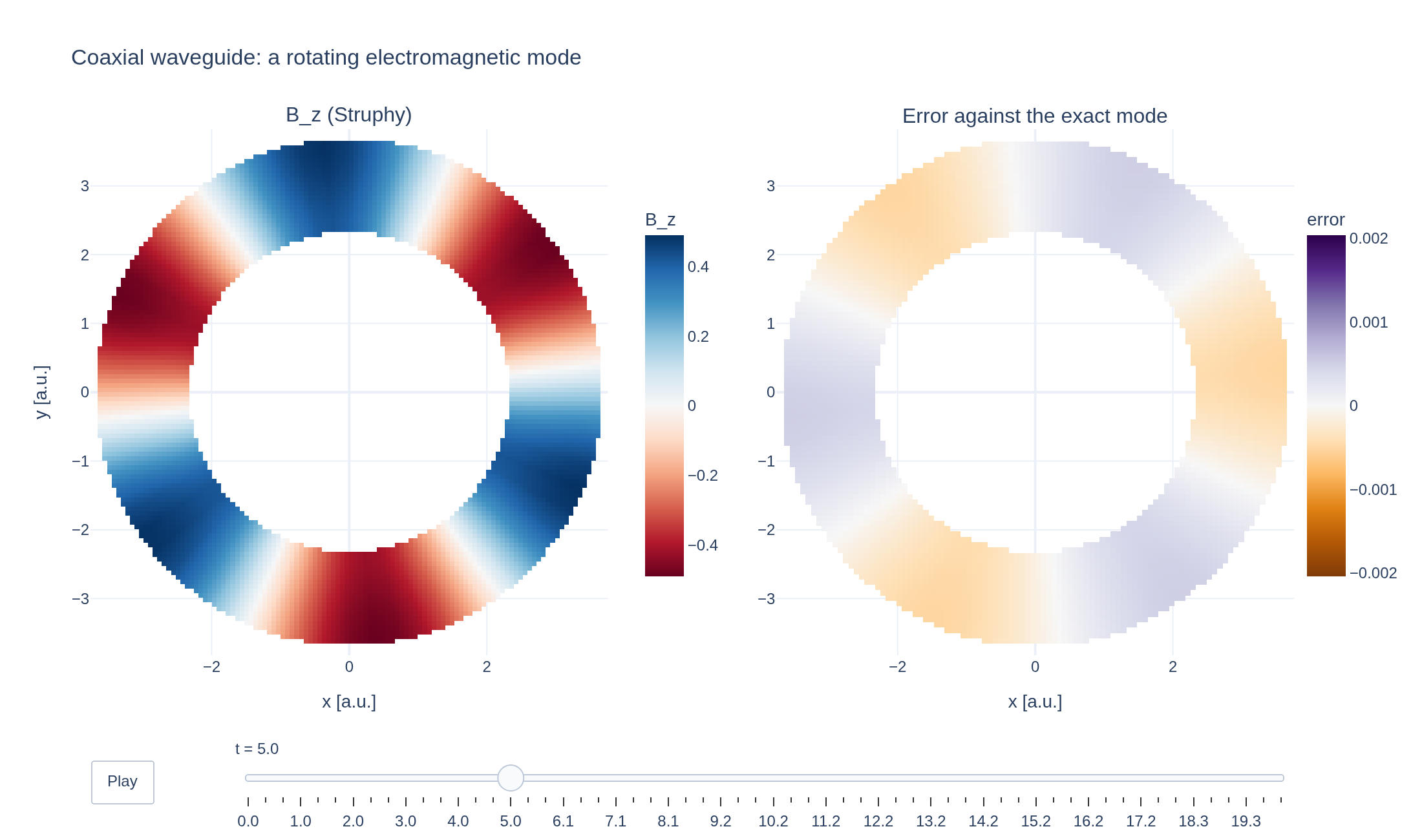


Physical problem
A rotating mode between conducting cylinders
Two perfectly conducting cylinders bound an annular domain with no axial variation. The initial field is the m = 3 coaxial eigenmode used in Struphy’s Maxwell tutorial. Its radial profile is J₃(r) − 0.28 Y₃(r); the radii are chosen at zeros of the profile’s derivative so that the tangential electric field vanishes at the walls.
The axial magnetic field is proportional to cos(3θ − t). Its temporal angular frequency is 1, while the pattern rotates at angular speed 1/3. The implicit Maxwell integrator evolves the fields for 400 steps. The comparison below separates phase error from energy conservation; conserving energy alone does not guarantee the correct frequency. The displayed maps interpolate the evaluated spline fields onto Cartesian pixels and mask the region outside the annulus.
PDEs solved by model:
Ampère's law (no current):
Faraday's law:
- Model
- Maxwell
- Grid
- 32 × 64 × 1
- FEEC degree
- 3 × 3 × 1
- Integrator
- Implicit
- Evolution
- 400 steps
- Visualization
- Plotly
Performance
Profiling
Struphy's built-in scope-profiler instruments every propagator, pusher and solver call — these are the real per-call timings from the run above, rendered live from its data.
Gantt (rank 0)
Region statistics
| Region | Count | Avg (s) | Min (s) | Max (s) | Total (s) |
|---|
Complete source
Run the simulation
Requires the Struphy revision pinned by this site, with compiled kernels, Plotly and Kaleido. Run struphy compile once, then execute python coaxial-waveguide.py.
"""Coaxial waveguide: an exact electromagnetic mode between two conducting cylinders.

Between two concentric perfectly conducting cylinders, Maxwell's equations have exact eigenmodes.
For azimuthal number m = 3 and no axial variation, the fields are a Bessel-function profile in the
radius times cos(m*theta - t): a pattern that rotates rigidly at frequency omega = 1. Struphy's
finite element Maxwell solver on the annulus is compared with this solution.

Adapted from Struphy's tutorial (tutorials/tutorial_maxwell.ipynb) and its verification test.

Requires Struphy 3.2 with compiled kernels (`struphy compile`).
"""

import numpy as np
import plotly.graph_objects as go
from plotly.subplots import make_subplots
from scipy.ndimage import map_coordinates
from scipy.optimize import curve_fit
from scipy.special import jv, yn

from struphy import DerhamOptions, EnvironmentOptions, Simulation, Time, domains, equils, grids, perturbations
from struphy.models import Maxwell

# The inner and outer radii are two zeros of the derivative of the radial profile
# J_m(r) - 0.28 Y_m(r), so that the tangential electric field vanishes on both conducting walls.
inner_radius = 2.326744
outer_radius = 3.686839
length = 2.0
mode_number = 3
bessel_ratio = 0.28

model = Maxwell()
model.propagators.maxwell.options = model.propagators.maxwell.Options(algo="implicit")
model.em_fields.e_field.add_perturbation(
    perturbations.CoaxialWaveguideElectric_r(m=mode_number, a1=inner_radius, a2=outer_radius)
)
model.em_fields.e_field.add_perturbation(
    perturbations.CoaxialWaveguideElectric_theta(m=mode_number, a1=inner_radius, a2=outer_radius)
)
model.em_fields.b_field.add_perturbation(
    perturbations.CoaxialWaveguideMagnetic(m=mode_number, a1=inner_radius, a2=outer_radius)
)

# The annulus in the (x, y) plane, with conducting walls (Dirichlet conditions) in the radial direction.
domain = domains.HollowCylinder(a1=inner_radius, a2=outer_radius, Lz=length)
grid = grids.TensorProductGrid(num_elements=(32, 64, 1))
derham_opts = DerhamOptions(degree=(3, 3, 1), bcs=(("dirichlet", "dirichlet"), None, None))

env = EnvironmentOptions(
    out_folders="struphy_gallery_runs",
    sim_folder="coaxial_waveguide",
)
sim = Simulation(
    model=model,
    name="Coaxial waveguide",
    description=(
        "An exact electromagnetic mode between two concentric conducting cylinders "
        "rotates around the annulus. Struphy's structure-preserving Maxwell solver "
        "reproduces its shape, its frequency and the conservation of its energy."
    ),
    env=env,
    time_opts=Time(dt=0.05, Tend=20.0),
    domain=domain,
    equil=equils.HomogenSlab(),
    grid=grid,
    derham_opts=derham_opts,
)

if __name__ == "__main__":
    from _gallery import export_profiling, merge_metadata, publish_thumbnail, save_extra_figure, save_figure

    output = sim.run(profiling_activated=True)
    output.pproc(physical=True)

    # The axial magnetic field on the (r, theta) evaluation grid, and the exact mode at the same points.
    b_z = output.evaluate("em_fields/b_field_xyz").isel(component=2, e3=0)  # (t, e1, e2)
    times = b_z.t.values
    radius = np.hypot(b_z.X.values, b_z.Y.values)
    angle = np.arctan2(b_z.Y.values, b_z.X.values)

    def exact_b_z(time):
        profile = jv(mode_number, radius) - bessel_ratio * yn(mode_number, radius)
        return profile * np.cos(mode_number * angle - time)

    error = np.stack([b_z.isel(t=index).values - exact_b_z(times[index]) for index in range(len(times))])
    amplitude = float(np.abs(exact_b_z(0.0)).max())
    relative_error = np.abs(error).max(axis=(1, 2)) / amplitude
    print(f"Largest relative error of B_z: {relative_error.max():.2e}")

    # The mode's frequency, from a sinusoid fitted to B_z at a probe in the middle of the gap. The
    # exact mode is proportional to cos(m theta - t), so its frequency is 1.
    probe = (b_z.sizes["e1"] // 2, 0)
    signal = b_z.values[:, probe[0], probe[1]]
    exact_signal = exact_b_z(times[:, None, None])[:, probe[0], probe[1]]
    fit, _ = curve_fit(lambda t, a, w, phase: a * np.cos(w * t + phase), times, signal, p0=[signal.max(), 1.0, 0.0])
    measured_frequency = float(fit[1])
    frequency_error = abs(measured_frequency - 1.0)
    print(f"Measured frequency: {measured_frequency:.5f} (exact: 1, error {frequency_error:.1e})")

    energy = output.evaluate("total_energy")
    energy_drift = float(np.abs(energy.values / energy.values[0] - 1.0).max())
    print(f"Largest relative change of the total energy: {energy_drift:.1e}")
    electric = output.evaluate("electric_energy")
    magnetic = output.evaluate("magnetic_energy")
    field_energy_variation = max(float((s.max() - s.min()) / s.mean()) for s in (electric, magnetic))

    # The animation: both fields are interpolated from the (r, theta) grid onto a Cartesian grid of
    # pixels, which are left empty outside the annulus. Every frame is embedded in the page, so the
    # smooth error map gets fewer pixels than the field.
    def pixel_grid(pixels):
        axis = np.linspace(-outer_radius, outer_radius, pixels)
        pixel_x, pixel_y = np.meshgrid(axis, axis)
        pixel_radius = np.hypot(pixel_x, pixel_y)
        pixel_angle = np.mod(np.arctan2(pixel_y, pixel_x), 2.0 * np.pi)
        outside = (pixel_radius < inner_radius) | (pixel_radius > outer_radius)
        index_r = (pixel_radius - inner_radius) / (outer_radius - inner_radius) * (b_z.sizes["e1"] - 1)
        index_theta = pixel_angle / (2.0 * np.pi) * (b_z.sizes["e2"] - 1)
        return axis, outside, index_r, index_theta

    def on_pixels(values, grid):
        _, outside, index_r, index_theta = grid
        image = map_coordinates(values, [index_r, index_theta], order=1, mode="nearest").astype(np.float32)
        image[outside] = np.nan
        return image

    field_grid = pixel_grid(112)
    error_grid = pixel_grid(96)

    frame_indices = np.linspace(0, len(times) - 1, 60, dtype=int)
    error_limit = float(np.abs(error).max())

    def frame_traces(index):
        return [
            go.Heatmap(
                z=on_pixels(b_z.isel(t=index).values, field_grid),
                x=field_grid[0],
                y=field_grid[0],
                zmin=-amplitude,
                zmax=amplitude,
                colorscale="RdBu",
                colorbar={"title": "B_z", "x": 0.45, "len": 0.75},
                xaxis="x",
                yaxis="y",
            ),
            go.Heatmap(
                z=on_pixels(error[index], error_grid),
                x=error_grid[0],
                y=error_grid[0],
                zmin=-error_limit,
                zmax=error_limit,
                colorscale="PuOr",
                colorbar={"title": "error", "x": 1.0, "len": 0.75, "exponentformat": "e"},
                xaxis="x2",
                yaxis="y2",
            ),
        ]

    figure = make_subplots(
        rows=1, cols=2, subplot_titles=("B_z (Struphy)", "Error against the exact mode"), horizontal_spacing=0.14
    )
    first, second = frame_traces(0)
    figure.add_trace(first, row=1, col=1)
    figure.add_trace(second, row=1, col=2)
    frames = [go.Frame(name=f"{times[index]:.1f}", data=frame_traces(index), traces=[0, 1]) for index in frame_indices]
    figure.frames = frames
    limit = 1.02 * outer_radius
    figure.update_xaxes(range=[-limit, limit], constrain="domain", title_text="x [a.u.]")
    figure.update_yaxes(range=[-limit, limit], title_text="y [a.u.]", row=1, col=1)
    figure.update_yaxes(range=[-limit, limit], row=1, col=2)
    figure.update_yaxes(scaleanchor="x", scaleratio=1, row=1, col=1)
    figure.update_yaxes(scaleanchor="x2", scaleratio=1, row=1, col=2)
    figure.update_layout(
        title="Coaxial waveguide: a rotating electromagnetic mode",
        template="plotly_white",
        autosize=True,
        margin={"l": 70, "r": 30, "t": 100, "b": 130},
        updatemenus=[
            {
                "type": "buttons",
                "showactive": False,
                "x": 0.0,
                "xanchor": "left",
                "y": -0.2,
                "yanchor": "top",
                "buttons": [
                    {
                        "label": "Play",
                        "method": "animate",
                        "args": [None, {"frame": {"duration": 60, "redraw": True}, "fromcurrent": True}],
                    },
                ],
            },
        ],
        sliders=[
            {
                "steps": [
                    {
                        "args": [[frame.name], {"frame": {"duration": 0, "redraw": True}, "mode": "immediate"}],
                        "label": frame.name,
                        "method": "animate",
                    }
                    for frame in frames
                ],
                "active": 0,
                "x": 0.12,
                "len": 0.88,
                "y": -0.1,
                "currentvalue": {"prefix": "t = "},
            },
        ],
    )

    # The still image and thumbnail show the mode a little after the start of the run.
    still_position = len(frame_indices) // 4
    save_figure(
        figure,
        "coaxial-waveguide",
        height=650,
        static_data=frame_traces(frame_indices[still_position]),
        static_active=still_position,
    )

    # The probe signal against the exact mode.
    probe_figure = go.Figure()
    probe_figure.add_scatter(
        x=times, y=exact_signal, mode="lines", name="exact mode", line={"color": "#d62828", "width": 3, "dash": "dot"}
    )
    probe_figure.add_scatter(x=times, y=signal, mode="lines", name="Struphy", line={"color": "#168aad", "width": 3})
    probe_figure.update_layout(
        title=f"Coaxial waveguide: B_z at a probe, measured frequency {measured_frequency:.4f} (exact: 1)",
        xaxis_title="t [a.u.]",
        yaxis_title="B_z at the probe [a.u.]",
        template="plotly_white",
        autosize=True,
        legend={"orientation": "h", "x": 0.5, "xanchor": "center", "y": 1.0, "yanchor": "bottom"},
        margin={"l": 70, "r": 30, "t": 110, "b": 60},
    )

    # The energies, and the relative change of the total energy.
    energy_figure = make_subplots(
        rows=2,
        cols=1,
        shared_xaxes=True,
        vertical_spacing=0.1,
        subplot_titles=("Energies", "Relative change of the total energy"),
    )
    for name, series, color, dash in (
        ("electric", electric, "#168aad", "solid"),
        ("magnetic", magnetic, "#f77f00", "dash"),
        ("total", energy, "#111111", "solid"),
    ):
        energy_figure.add_scatter(
            x=times,
            y=series.values,
            mode="lines",
            name=name,
            line={"color": color, "width": 3, "dash": dash},
            row=1,
            col=1,
        )
    energy_figure.add_scatter(
        x=times,
        y=np.abs(energy.values / energy.values[0] - 1.0) + 1e-17,
        mode="lines",
        showlegend=False,
        line={"color": "#111111", "width": 2},
        row=2,
        col=1,
    )
    energy_figure.update_yaxes(title_text="energy [a.u.]", rangemode="tozero", row=1, col=1)
    energy_figure.update_yaxes(
        title_text="|ΔW / W₀|", type="log", dtick=1, exponentformat="power", range=[-16, -13], row=2, col=1
    )
    energy_figure.update_xaxes(title_text="t [a.u.]", row=2, col=1)
    energy_figure.update_layout(template="plotly_white", autosize=True, margin={"l": 80, "r": 30, "t": 80, "b": 60})

    figures = [
        save_extra_figure(
            probe_figure,
            "coaxial-waveguide",
            "frequency",
            alt="Axial magnetic field at a probe against the exact coaxial mode",
            caption=(
                "The axial magnetic field at a fixed probe in the middle of the gap, from Struphy and from the exact "
                f"mode, which is proportional to cos(3θ − t). A sinusoid fitted to the Struphy signal has frequency "
                f"{measured_frequency:.5f} against the exact value 1, a relative error of {frequency_error:.1e}. This "
                f"phase drift is the source of the field error of the animation: {frequency_error * times[-1]:.1e} "
                f"of the mode amplitude at t = {times[-1]:.0f}, against the measured maximum of {relative_error.max():.1e}."
            ),
        ),
        save_extra_figure(
            energy_figure,
            "coaxial-waveguide",
            "energy",
            alt="Electric, magnetic and total energy of the coaxial mode against time",
            caption=(
                "The electric and magnetic energies of the rotating mode are equal and constant to about "
                f"{field_energy_variation:.0e} (relative), since the energy density pattern rotates with the mode, and so "
                f"is their sum. The relative change of the total energy, below, stays under {energy_drift:.0e} over "
                f"{len(times) - 1} steps: the implicit time integrator conserves the energy to round-off."
            ),
        ),
    ]

    profiling = export_profiling(sim, "coaxial-waveguide")

    merge_metadata(
        "coaxial-waveguide",
        measuredFrequency=measured_frequency,
        exactFrequency=1.0,
        frequencyError=frequency_error,
        maxRelativeError=float(relative_error.max()),
        energyDrift=energy_drift,
        modeNumber=mode_number,
        figures=figures,
        **publish_thumbnail("coaxial-waveguide"),
        **profiling,
    )
Adapted from Struphy’s Maxwell tutorial and its analytic coaxial perturbations.