Overview

This model simulates the propagation of electromagnetic waves in vacuum

using Maxwell's equations without sources. It uses a finite element exterior calculus (FEEC) formulation with the electric field in H(curl) and the magnetic field in H(div) spaces.

Use cases

Propagation of electromagnetic waves in vacuum.

Governing equations

PDEs solved by model:

Ampère's law (no current):

\frac{\partial E}{\partial t} - \nabla \times B = 0

Faraday's law:

\frac{\partial B}{\partial t} + \nabla \times E = 0

Normalization

Velocity and fields are normalized as:

v^= c, E^= c B^

where $c$ is the speed of light.

Discretization

Time integration is performed by the following propagators (in sequence):

MaxwellWeakAmpere

Diagnostics

The following scalars are tracked during simulation:

Electric energy: $E_{E} = \frac{1}{2} \int ∣ E ∣^{2} d V$
Magnetic energy: $E_{B} = \frac{1}{2} \int ∣ B ∣^{2} d V$
Total energy: $E_{t o t a l} = E_{E} + E_{B}$

Examples

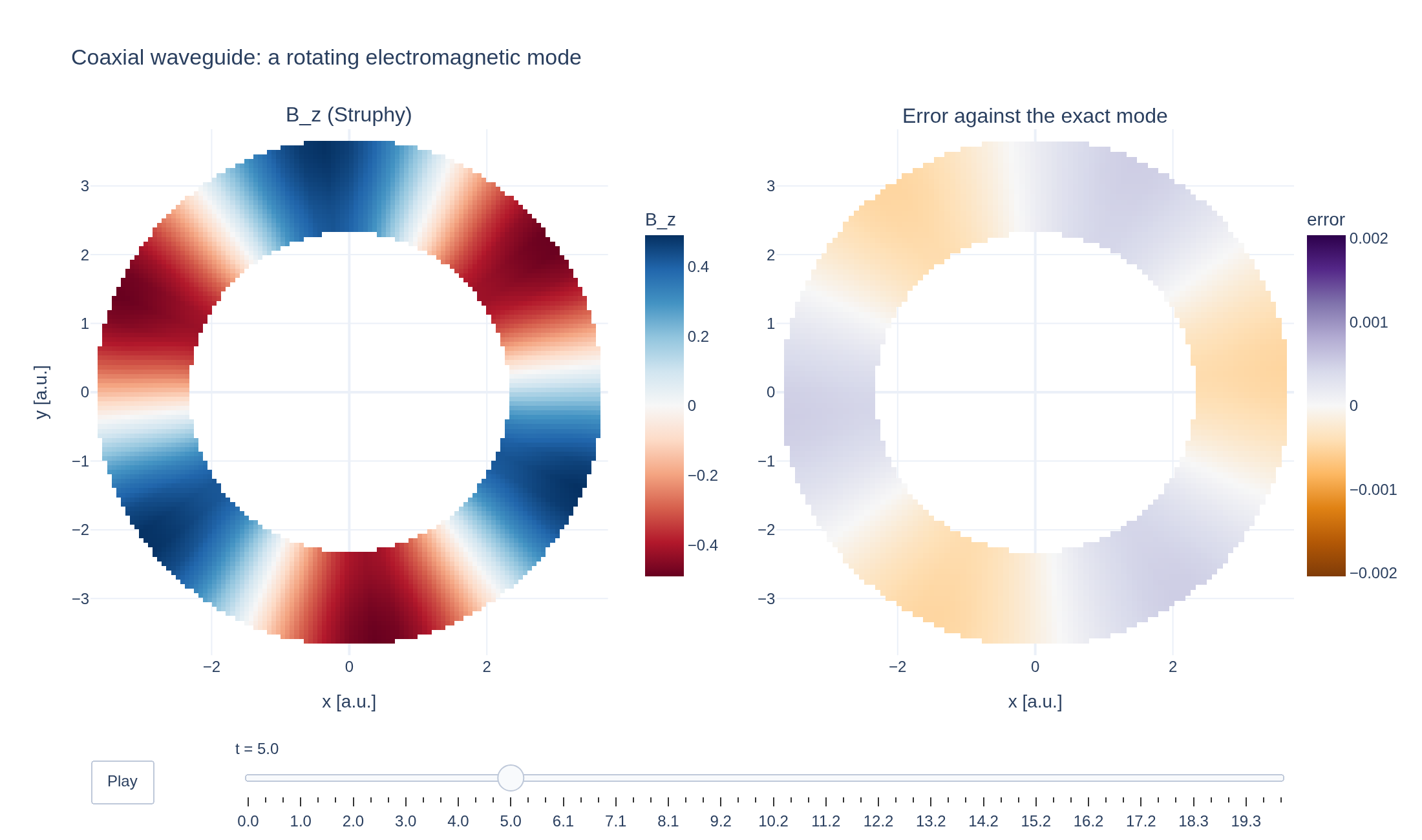
Coaxial waveguide

An exact electromagnetic mode between two concentric conducting cylinders rotates around the annulus. Struphy's structure-preserving Maxwell solver reproduces its shape, its frequency and the conservation of its energy. With $F(r)=J_3(r)-0.28Y_3(r)$ , the initial mode is $E_r=-\frac{3F(r)}{r}\cos(3\theta),\qquad E_\theta=F\prime(r)\sin(3\theta),\qquad B_z=F(r)\cos(3\theta),$ between $r=2.326744$ and $r=3.686839$ ; $J_3$ and $Y_3$ are Bessel functions.

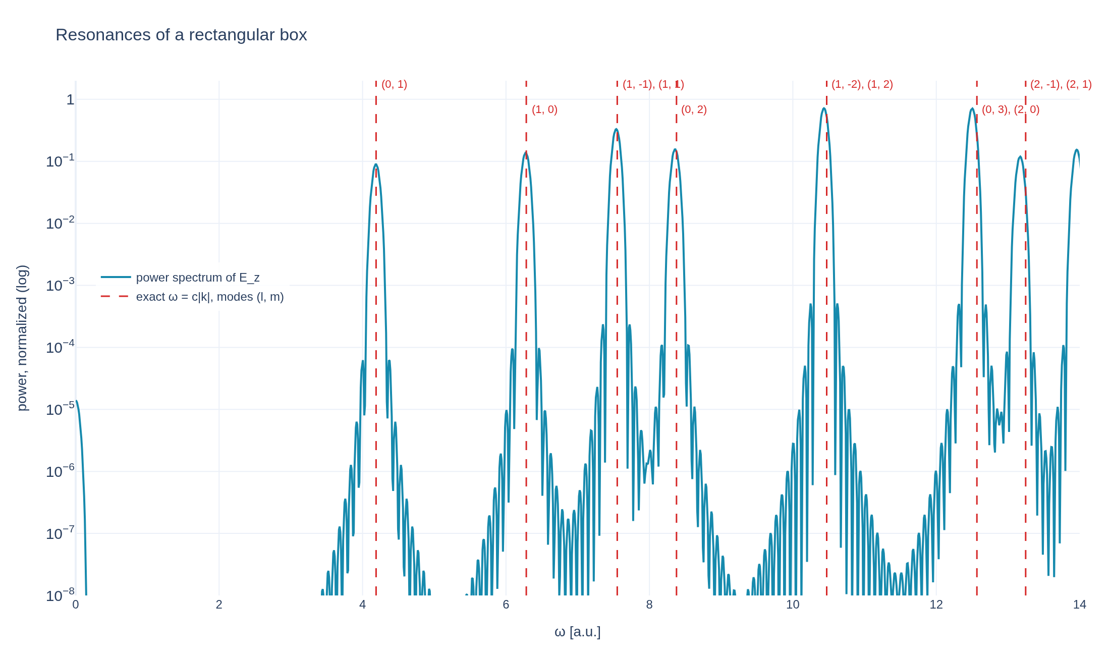
Maxwell cavity resonances

Noise in the electric field excites every electromagnetic mode of a rectangular periodic box. The power spectrum of the field over time has one peak per resonance, at the exact frequencies ω = c |k| of the box. The launch uses $E_z$ coefficient noise of amplitude $0.1$ and $\mathbf{B}(x,y,0)=0$ . The periodic box selects $\mathbf{k}_{mn}=2\pi\left(\frac{m}{L_x},\frac{n}{L_y}\right),\qquad (L_x,L_y)=(1,1.5),$ for integer mode numbers $m,n$ .

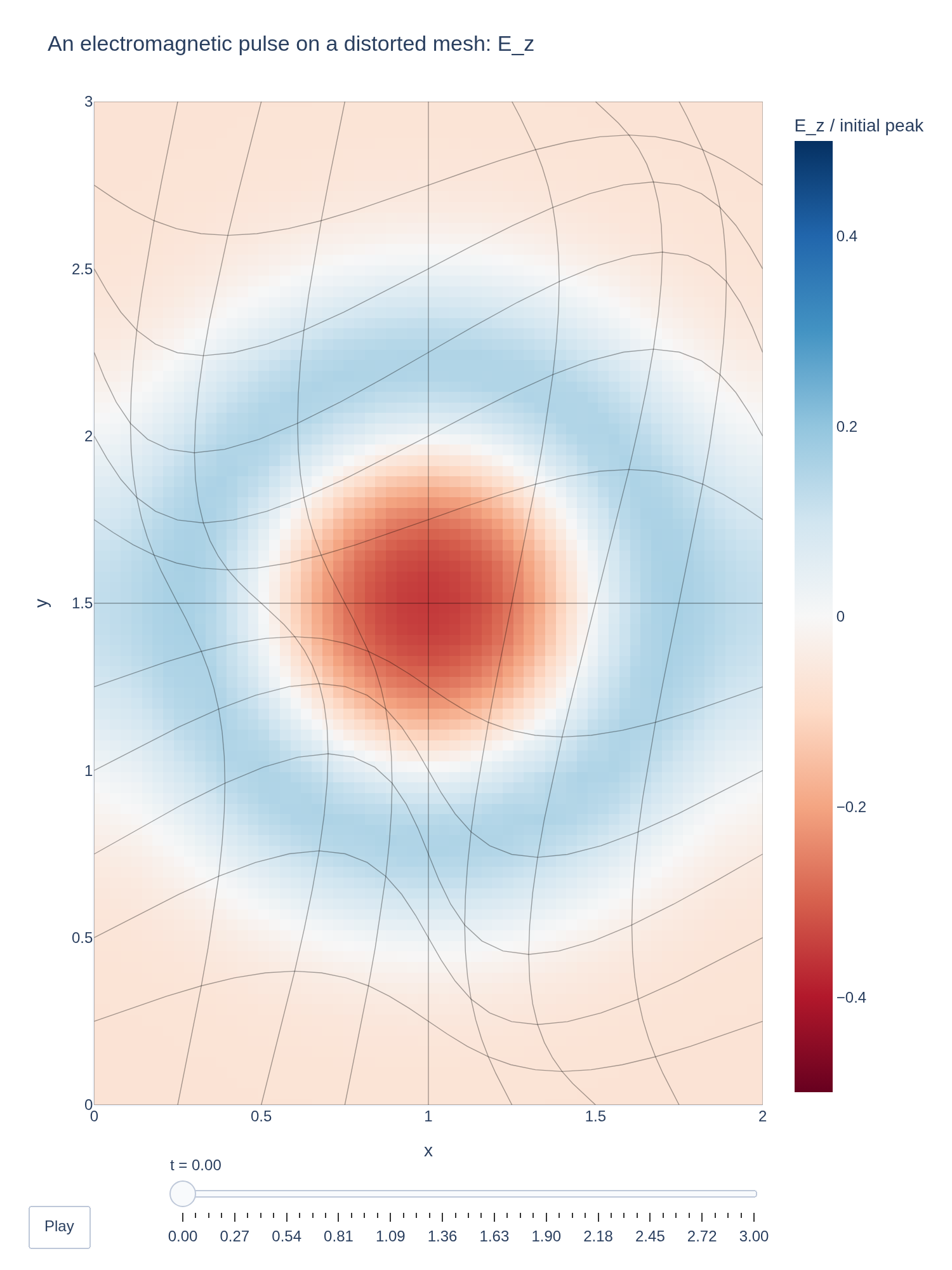
Electromagnetic pulse on a distorted mesh

A Gaussian pulse of the electric field spreads as a ring across a periodic box, on a mesh that the Colella mapping has bent. The structure-preserving Maxwell solver keeps the energy constant and follows the exact solution, which is a sum of cosine modes. The initial pulse is a truncated, zero-mean Gaussian Fourier expansion: $E_z(x,y,0)=\sum_{\substack{0\le l,m\le6\\(l,m)\ne(0,0)}}a_{lm}\cos[k_l(x-1)]\cos[q_m(y-1.5)],$ where $k_l=\pi l$ , $q_m=2\pi m/3$ and $a_{lm}=(2-\delta_{l0})(2-\delta_{m0})(2\pi\sigma^2/6)e^{-\sigma^2(k_l^2+q_m^2)/2}$ . The width is $\sigma=0.25$ , $\delta_{ij}$ is the Kronecker delta, and the magnetic field starts at zero.

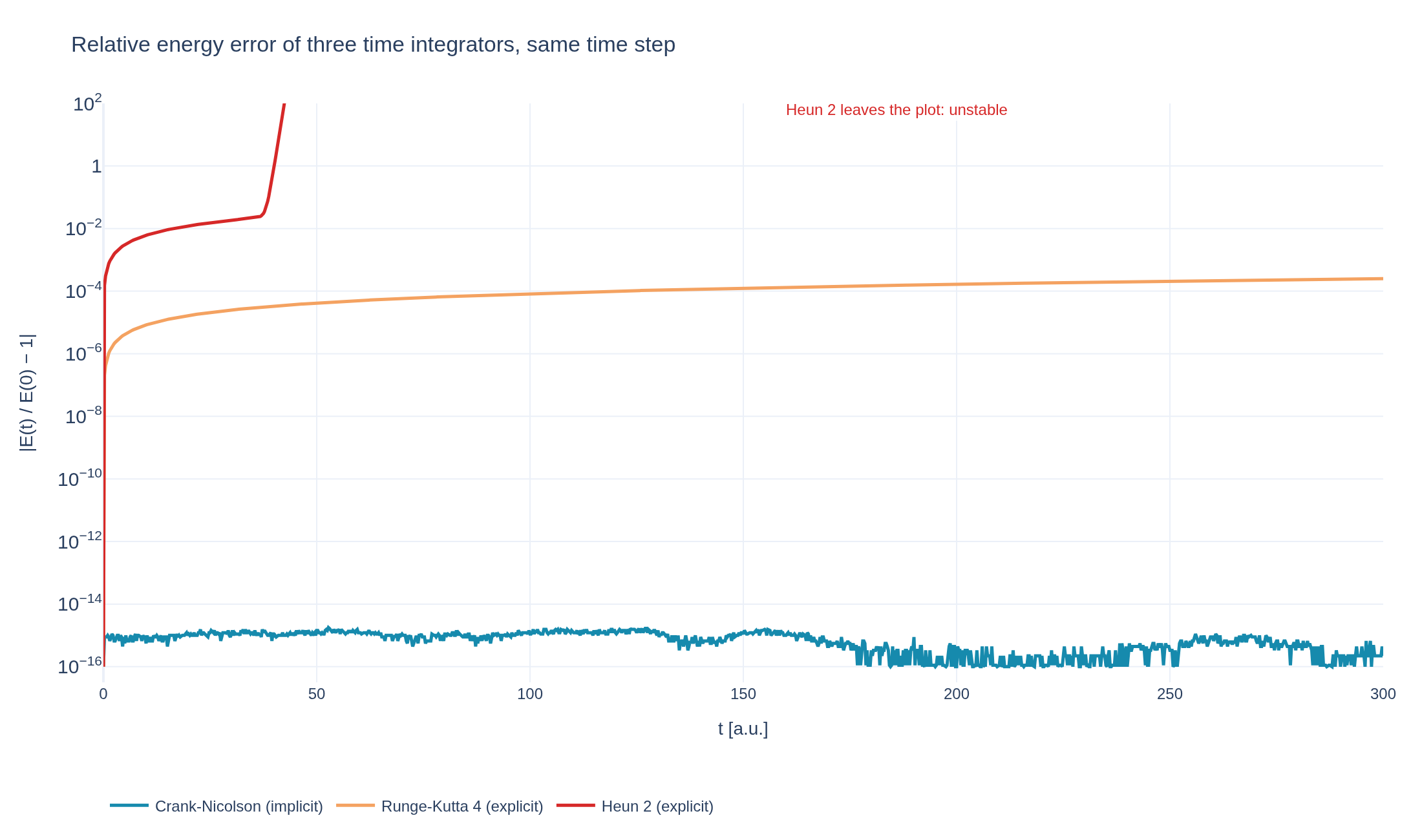
Structure preservation in time integration

One standing electromagnetic wave, stepped by Crank-Nicolson, RK4 and Heun's method at the same time step. The symplectic implicit scheme keeps the energy error bounded for the whole run, while the explicit schemes do not: RK4 loses energy steadily, and Heun's method is unstable for this operator. All three runs start from $\mathbf{E}(z,0)=(0.1\sin(\pi z/5),0,0),\qquad \mathbf{B}(z,0)=0,$ with periodic length $L_z=20$ and time step $\Delta t=0.25$ in units where $c=1$ .

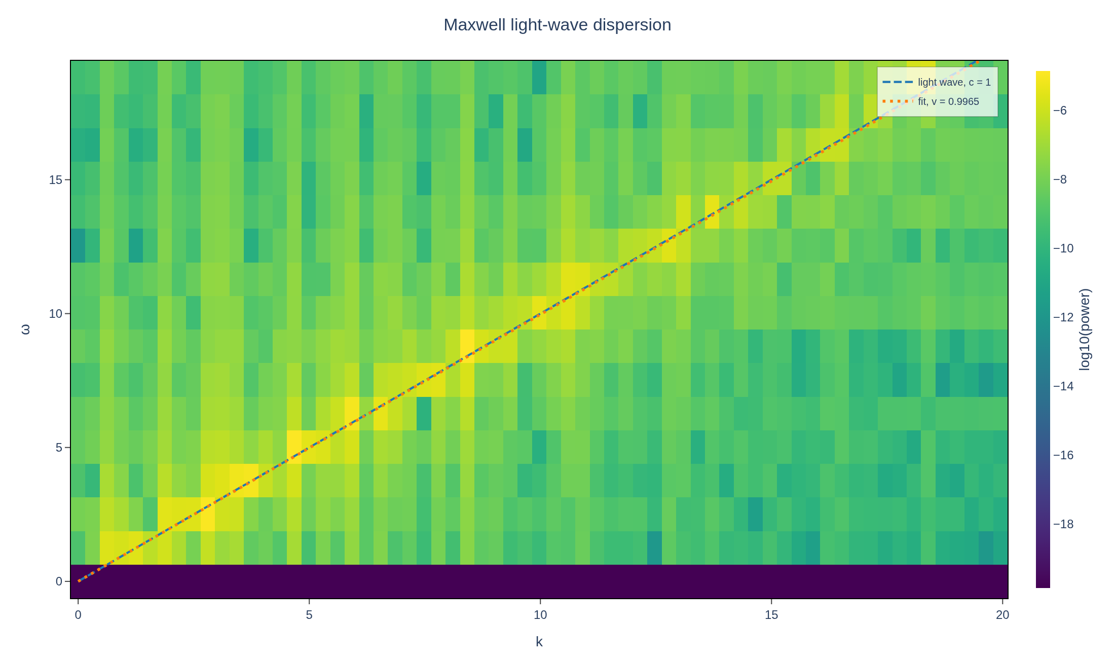
Maxwell light-wave dispersion

Excite a broadband electric field and recover the vacuum dispersion relation ω = ck with Struphy’s FEEC Maxwell solver. The two transverse electric components start with coefficient-noise amplitude $A=0.1$ , while $\mathbf{B}(z,0)=0$ . On the periodic interval $L_z=20$ , the allowed wavenumbers are $k_n=\frac{2\pi n}{20},\qquad n\in\mathbb{Z}.$