Dam break

A dense fluid column collapses under gravity in a closed box. Smoothed particle hydrodynamics follows the collapse, the wave across the box and the settling of the fluid, using markers alone.

← All examples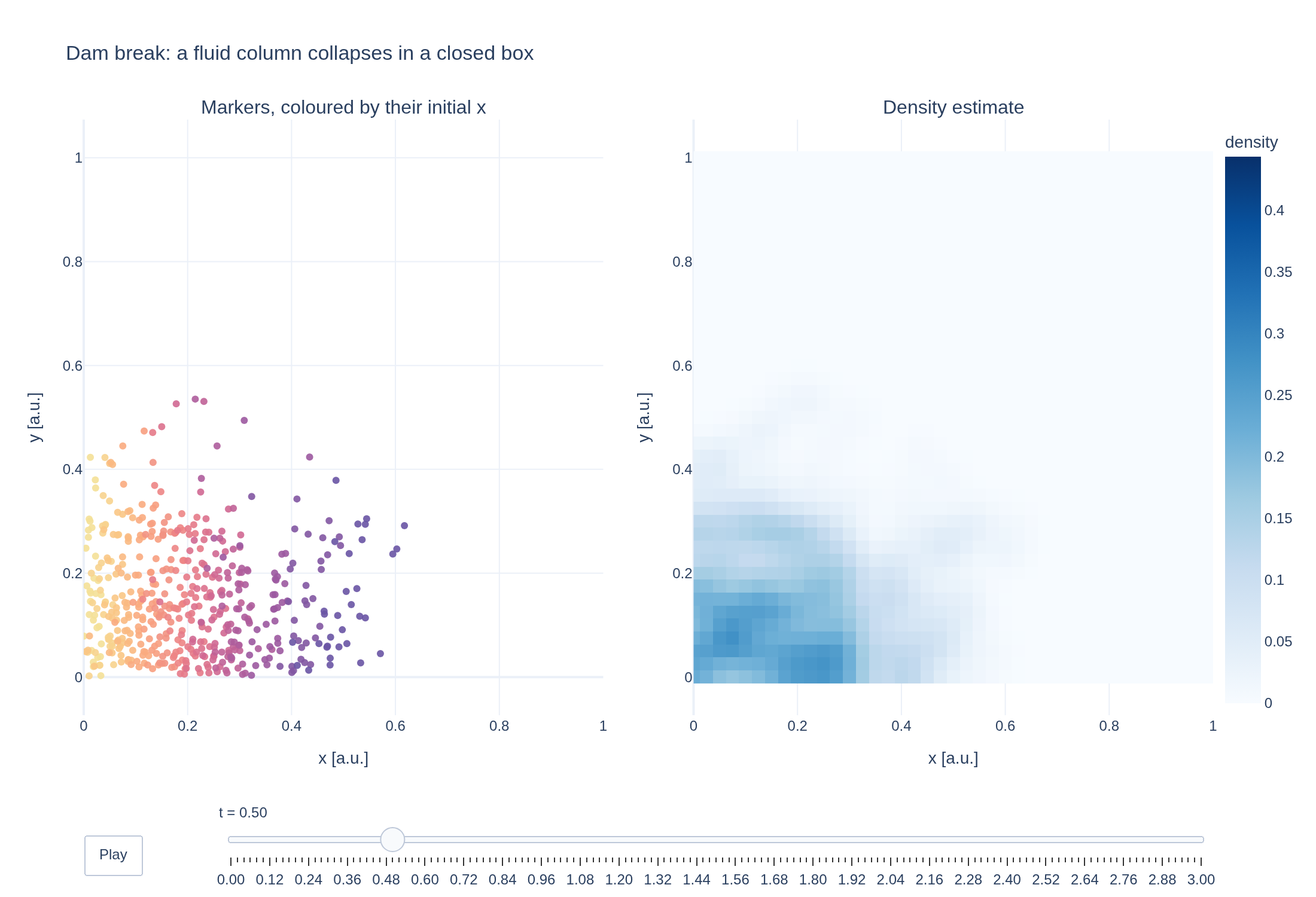

Actual output from the script below: 512 SPH markers (left, coloured by where they started in the column) and the density estimated from them (right). Press Play or drag the slider to follow the collapse; the still image shows t = 0.5. The front of the fluid reaches the far wall at t ≈ 0.76, and no marker leaves the closed box during the run.

The front of the fluid (the largest marker x) and the height of its centre of mass. The front reaches the far wall at t ≈ 0.76 and stays there. The centre of mass falls from 0.5 to about 0.15 by t ≈ 0.4, close to the free-fall time of 0.32, rises slightly as the fluid rebounds, and then settles slowly towards a layer at the bottom.

Physical problem

A fluid column released in a closed box

A dense fluid column fills the left quarter of a unit box with reflecting walls and is released at t = 0. Gravity pulls it down, and the pressure gradient drives a wave across the bottom of the box towards the far wall. The fluid is followed by markers alone: each marker carries mass, and the density is estimated from the markers with a smoothing kernel, so the free surface needs no special treatment.

The pressure is isothermal, p = κρ with κ = 0.2 (sound speed about 0.45), a weakly compressible model with a little viscosity (μ = 0.05) for stability. Gravity is 10, so the free-fall time from mid-height is about 0.32. With this small κ the fluid is quite compressible: the density estimate rises from 0.1 in the column to about 0.4 at the bottom of the box. The box is loaded uniformly with almost no weight outside the column, and those markers are removed before the run; mirror ghost markers enforce the reflecting walls.

PDEs solved by model:

Continuity:

\partial_{t} ρ + \nabla \cdot (ρ u) = 0

Momentum:

ρ (\partial_{t} u + u \cdot \nabla u) = - \nabla (ρ^{2} \frac{\partial U ( ρ , S )}{\partial ρ}) - \nabla \cdot π

Entropy:

\partial_{t} S + u \cdot \nabla S = 0

where $S$ denotes the entropy per unit mass and $π$ is the viscous stress tensor.

The viscous stress tensor for a Newtonian fluid is given by:

σ = - μ (\nabla u + (\nabla u)^{T} - \frac{2}{3} (\nabla \cdot u) I)

where $μ$ is the dynamic (shear) viscosity and $I$ is the identity tensor.

The internal energy per unit mass can be defined in two ways:

isothermal : U (ρ, S) = κ (S) lo g ρ

polytropic : U (ρ, S) = κ (S) \frac{ρ ^{γ - 1}}{γ - 1}

Model: ViscousEulerSPH
Domain: Cuboid
Markers: 512
SPH kernel: Gaussian, 2D
Integrator: Forward euler
Evolution: 150 steps
Visualization: Plotly

Performance

Profiling

Download profile .h5

Struphy's built-in scope-profiler instruments every propagator, pusher and solver call — these are the real per-call timings from the run above, rendered live from its data.

Durations

Gantt (rank 0)

Region statistics

Region	Count	Avg (s)	Min (s)	Max (s)	Total (s)

Complete source

Run the simulation

Download .py

Requires Struphy 3.2 with compiled kernels and Plotly. Run struphy compile once, then execute python dam-break.py.

"""Dam break: a fluid column collapses under gravity in a closed box.

A dense fluid column fills the left quarter of a closed, two-dimensional box and
is released at t = 0. Gravity pulls it down, the pressure gradient drives a wave
across the box, and the fluid runs up the far wall, splashes back and sloshes
until it settles in a layer at the bottom. Smoothed particle hydrodynamics (SPH)
follows the free surface with markers alone, without a grid.

Adapted from Struphy's tutorial (tutorials/tutorial_dam_break_sph.ipynb).

Requires Struphy 3.2 with compiled kernels (`struphy compile`).
"""

import numpy as np
import plotly.graph_objects as go
from plotly.subplots import make_subplots

from struphy import (
    BoundaryParameters,
    EnvironmentOptions,
    KernelDensityPlot,
    LoadingParameters,
    SavingParameters,
    Simulation,
    SortingParameters,
    Time,
    WeightsParameters,
    domains,
    equils,
)
from struphy.models import ViscousEulerSPH
from struphy.ode.utils import ButcherTableau

# Weakly compressible SPH: the isothermal pressure p = kappa * rho, with kappa = c_s^2 small
# enough that the flow stays roughly subsonic, and a little viscosity for stability.
kappa = 0.2
viscosity = 0.05
gravity = 10.0
column_density = 0.1
boxes_per_dimension = 8
markers_per_box = 32
density_points = 41

model = ViscousEulerSPH(with_B0=False, with_p=True, with_viscosity=True)
model.propagators.push_eta.options = model.propagators.push_eta.Options(
    butcher=ButcherTableau(algo="forward_euler"),
)
model.propagators.push_sph_p.options = model.propagators.push_sph_p.Options(
    kernel_type="gaussian_2d",
    gravity=(0.0, -gravity, 0.0),
    kappa=kappa,
)
model.propagators.push_viscous.options = model.propagators.push_viscous.Options(
    kernel_type="gaussian_2d",
    mu=viscosity,
)

# A closed box of unit size with reflecting walls, and mirror ghost markers for the SPH kernels.
domain = domains.Cuboid(r1=1.0, r2=1.0)
model.euler_fluid.set_markers(
    loading_params=LoadingParameters(ppb=markers_per_box, loading="tesselation"),
    # The box is loaded uniformly with almost no weight outside the column; those markers are removed.
    weights_params=WeightsParameters(reject_weights=True, threshold=1e-6),
    boundary_params=BoundaryParameters(bc=("reflect", "reflect", "periodic"), bc_sph=("mirror", "mirror", "periodic")),
    sorting_params=SortingParameters(
        boxes_per_dim=(boxes_per_dimension, boxes_per_dimension, 1), dims_mask=(True, True, False)
    ),
    # Save every marker at every step, and a kernel density estimate on a grid.
    saving_params=SavingParameters(
        n_markers=1.0,
        kernel_density_plots=(KernelDensityPlot(pts_e1=density_points, pts_e2=density_points, pts_e3=1),),
    ),
    bufsize=2,
)

# The dense column occupies x < 1/4; everywhere else the density is negligible.
model.euler_fluid.var.add_background(
    equils.ConstantVelocity(density_profile="step_function_xy", n=column_density, upper_x=0.25, upper_y=1.0),
)

env = EnvironmentOptions(
    out_folders="struphy_gallery_runs",
    sim_folder="dam_break",
)
sim = Simulation(
    model=model,
    name="Dam break",
    description=(
        "A dense fluid column collapses under gravity in a closed box. Smoothed "
        "particle hydrodynamics follows the collapse, the wave across the box and "
        "the settling of the fluid, using markers alone."
    ),
    env=env,
    time_opts=Time(dt=0.02, Tend=3.0, split_algo="Strang"),
    domain=domain,
    grid=None,
    derham_opts=None,
)

if __name__ == "__main__":
    from _gallery import export_profiling, merge_metadata, publish_thumbnail, save_extra_figure, save_figure

    output = sim.run(profiling_activated=True)
    output.pproc()

    density = output.evaluate("euler_fluid/view_0/n").isel(e3=0)  # (t, e1, e2)
    orbits = output.evaluate("euler_fluid")  # (t, marker, quantity); the first two quantities are x and y
    x = orbits.sel(quantity="x")
    y = orbits.sel(quantity="y")
    times = orbits.t.values

    # The front of the fluid and the height of its centre of mass, and a check that no marker
    # ever left the closed box (a small tolerance for the displacement within one step).
    front = x.max("marker")
    centre_of_mass = y.mean("marker")
    arrival_index = int(np.argmax(front.values >= 0.95))
    arrival_time = float(times[arrival_index])
    in_box = bool(((x >= -0.01) & (x <= 1.01) & (y >= -0.01) & (y <= 1.01)).all())
    print(f"Front reaches the far wall at t = {arrival_time:.2f}; all markers inside the box: {in_box}")

    # Colour each marker by where it started in the column, to follow the mixing.
    shade = x.isel(t=0).values / 0.25
    positions = density.e1.values  # the density is estimated on a grid over the unit box
    heights = density.e2.values
    density_limit = float(density.max())

    def frame_traces(index, webgl=True):
        # In an animation, plotly.js 3.7 stops drawing a heatmap that shares the figure with SVG scatter
        # frames, so the markers of the interactive figure are drawn with WebGL.
        markers = go.Scattergl if webgl else go.Scatter
        return [
            markers(
                x=x.isel(t=index).values,
                y=y.isel(t=index).values,
                mode="markers",
                marker={"size": 6, "color": shade, "colorscale": "Sunset", "cmin": 0.0, "cmax": 1.0, "opacity": 0.9},
                showlegend=False,
                xaxis="x",
                yaxis="y",
            ),
            go.Heatmap(
                z=density.isel(t=index).transpose("e2", "e1").values,
                x=positions,
                y=heights,
                zmin=0.0,
                zmax=density_limit,
                colorscale="Blues",
                colorbar={"title": "density", "x": 1.0},
                xaxis="x2",
                yaxis="y2",
            ),
        ]

    figure = make_subplots(
        rows=1,
        cols=2,
        subplot_titles=("Markers, coloured by their initial x", "Density estimate"),
        horizontal_spacing=0.08,
    )
    scatter, heatmap = frame_traces(0)
    figure.add_trace(scatter, row=1, col=1)
    figure.add_trace(heatmap, row=1, col=2)
    frames = [
        go.Frame(name=f"{times[index]:.2f}", data=frame_traces(index), traces=[0, 1]) for index in range(len(times))
    ]
    figure.frames = frames
    figure.update_xaxes(range=[0, 1], constrain="domain", title_text="x [a.u.]")
    figure.update_yaxes(range=[0, 1], title_text="y [a.u.]")
    figure.update_yaxes(scaleanchor="x", scaleratio=1, row=1, col=1)
    figure.update_yaxes(scaleanchor="x2", scaleratio=1, row=1, col=2)
    figure.update_layout(
        title="Dam break: a fluid column collapses in a closed box",
        template="plotly_white",
        autosize=True,
        margin={"l": 70, "r": 30, "t": 100, "b": 130},
        updatemenus=[
            {
                "type": "buttons",
                "showactive": False,
                "x": 0.0,
                "xanchor": "left",
                "y": -0.2,
                "yanchor": "top",
                "buttons": [
                    {
                        "label": "Play",
                        "method": "animate",
                        "args": [None, {"frame": {"duration": 40, "redraw": True}, "fromcurrent": True}],
                    },
                ],
            },
        ],
        sliders=[
            {
                "steps": [
                    {
                        "args": [[frame.name], {"frame": {"duration": 0, "redraw": True}, "mode": "immediate"}],
                        "label": frame.name,
                        "method": "animate",
                    }
                    for frame in frames
                ],
                "active": 0,
                "x": 0.12,
                "len": 0.88,
                "y": -0.1,
                "currentvalue": {"prefix": "t = "},
            },
        ],
    )

    # The still image shows the collapse under way (t = 0.5) rather than the initial column.
    still_index = int(np.argmin(abs(times - 0.5)))
    save_figure(
        figure, "dam-break", height=750, static_data=frame_traces(still_index, webgl=False), static_active=still_index
    )

    trajectory = go.Figure()
    trajectory.add_scatter(
        x=times,
        y=front.values,
        mode="lines",
        name="front of the fluid (largest x)",
        line={"color": "#168aad", "width": 3},
    )
    trajectory.add_scatter(
        x=times,
        y=centre_of_mass.values,
        mode="lines",
        name="height of the centre of mass",
        line={"color": "#d62828", "width": 3},
    )
    trajectory.update_layout(
        title="Dam break: front and centre of mass",
        xaxis_title="t [a.u.]",
        yaxis_title="position in the box [a.u.]",
        template="plotly_white",
        autosize=True,
        legend={"x": 0.98, "y": 0.5, "xanchor": "right", "bgcolor": "rgba(255,255,255,0.82)"},
        margin={"l": 70, "r": 30, "t": 80, "b": 60},
    )
    figures = [
        save_extra_figure(
            trajectory,
            "dam-break",
            "front",
            alt="Position of the fluid front and height of the centre of mass over time",
            caption=(
                f"The front of the fluid (the largest marker x) and the height of its centre of mass. The front "
                f"reaches the far wall at t ≈ {arrival_time:.2f} and stays there. The centre of mass falls from 0.5 "
                "to about 0.15 by t ≈ 0.4, close to the free-fall time of 0.32, rises slightly as the fluid rebounds, "
                "and then settles slowly towards a layer at the bottom."
            ),
        ),
    ]

    profiling = export_profiling(sim, "dam-break")

    merge_metadata(
        "dam-break",
        arrivalTime=arrival_time,
        markers=int(x.sizes["marker"]),
        markersInBox=in_box,
        kernel="Gaussian, 2D",
        figures=figures,
        **publish_thumbnail("dam-break"),
        **profiling,
    )

Adapted from Struphy’s dam-break SPH tutorial. See the post-processing guide for more ways to inspect the result.