RandomParticleDiffusion · Diffusion
Random and deterministic particle diffusion
A cosine density relaxes by diffusion. Struphy's random-walk and deterministic particle methods both follow it, and their density and decay of the mode are compared with the exact solution.
Run the simulation ↓← All examples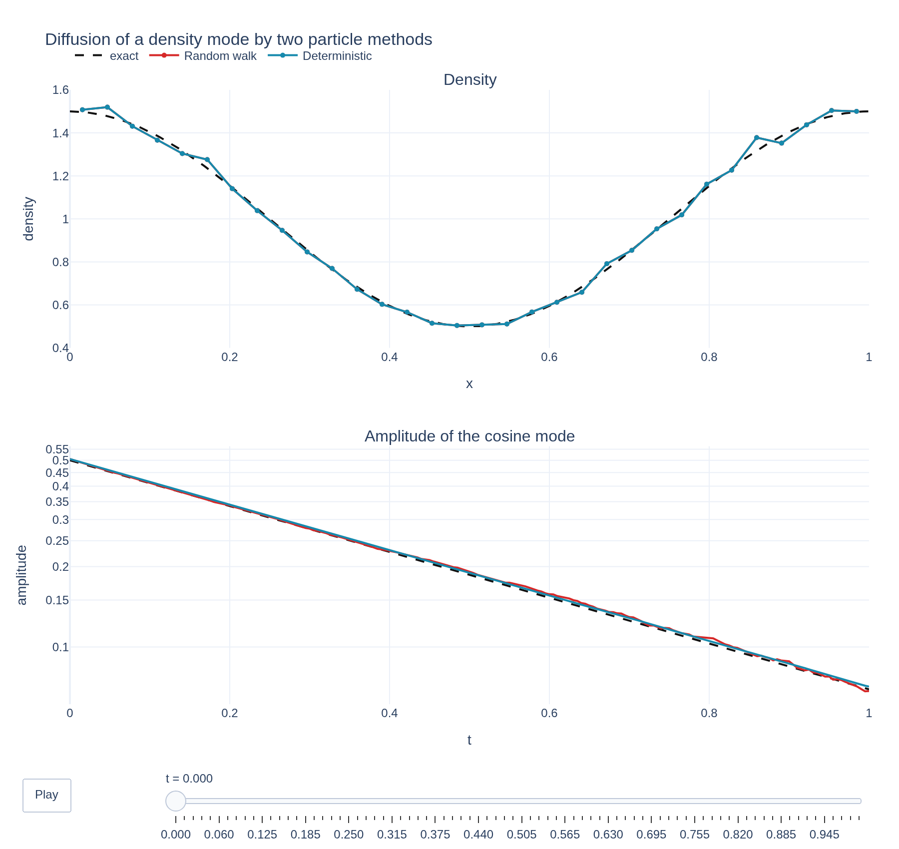
Physical problem
Diffusion with random and deterministic particles
A cosine density relaxes by diffusion. Struphy's random-walk and deterministic particle methods both follow it, and their density and decay of the mode are compared with the exact solution.
PDEs solved by model:
Find such that
where is a positive diffusion coefficient.
- Domain
- Cuboid
- Evolution
- 200 steps
- Visualization
- Plotly
Performance
Profiling
Struphy's built-in scope-profiler instruments every propagator, pusher and solver call — these are the real per-call timings from the run above.
Gantt (rank 0)
Region statistics
| Region | Count | Avg (s) | Min (s) | Max (s) | Total (s) |
|---|
Complete source
Run the simulation
Requires Struphy with compiled kernels and Plotly. Run struphy compile once, then execute python diffusion-methods.py.
"""Two particle methods for the diffusion equation: random walks and a deterministic drift.

A periodic density u(x, 0) = 1 + a cos(2 pi x) relaxes to the uniform state by diffusion,
du/dt = D u'', and the amplitude of the mode decays as a exp(-D k^2 t) with k = 2 pi. Struphy solves this
with particles in two ways:

* `RandomParticleDiffusion` moves every marker by a Wiener process, dx = sqrt(2 D) dB. The density is
  that of the markers, so the result is noisy, and the noise falls only as 1 / sqrt(N).
* `DeterministicParticleDiffusion` moves every marker with the velocity -D u'/u, where the density u is a
  finite element projection of the markers' own weights. There is no random noise, but the density
  estimate limits the accuracy.

Both start from the same markers and are compared with the exact decay.

Requires Struphy 3.3 with compiled kernels (`struphy compile`).
"""

import numpy as np
import plotly.graph_objects as go

from struphy import (
    BinningPlot,
    BoundaryParameters,
    DerhamOptions,
    EnvironmentOptions,
    LoadingParameters,
    SavingParameters,
    Simulation,
    Time,
    WeightsParameters,
    domains,
    grids,
    maxwellians,
    perturbations,
)
from struphy.models import DeterministicParticleDiffusion, RandomParticleDiffusion
from struphy.ode.utils import ButcherTableau

diffusion = 0.05  # D
amplitude = 0.5  # of the initial density perturbation, relative to the uniform density 1
wavenumber = 2 * np.pi
decay_rate = diffusion * wavenumber**2  # the exact decay rate of the mode
markers = 100_000
bins = 32
time_opts = Time(dt=0.005, Tend=1.0, split_algo="LieTrotter")

domain = domains.Cuboid(r1=1.0)
# The finite element grid is used only by the deterministic method, to estimate the density.
grid = grids.TensorProductGrid(num_elements=(32, 1, 1))
derham_opts = DerhamOptions(degree=(3, 1, 1))


def make_model(model_class, propagator_name, **options):
    """A diffusion model with the same markers and initial density, for either method."""
    model = model_class()
    model.hydrogen.set_markers(
        loading_params=LoadingParameters(Np=markers, loading="pseudo_random", seed=1608),
        weights_params=WeightsParameters(),
        boundary_params=BoundaryParameters(),
        saving_params=SavingParameters(
            binning_plots=(BinningPlot(slice="e1", n_bins=(bins,), ranges=(0.0, 1.0)),),
        ),
    )
    propagator = getattr(model.propagators, propagator_name)
    propagator.options = propagator.Options(diff_coeff=diffusion, **options)
    # A uniform background, and the cosine mode as the initial condition.
    model.hydrogen.var.add_background(maxwellians.ColdPlasma(n=(1.0, None)))
    mode = perturbations.ModesCos(amps=(amplitude,), ls=(1,))
    model.hydrogen.var.add_initial_condition(maxwellians.ColdPlasma(n=(1.0, mode)))
    return model


def make_simulation(model, folder, **extra):
    return Simulation(
        model=model,
        env=EnvironmentOptions(out_folders="struphy_gallery_runs", sim_folder=folder),
        time_opts=time_opts,
        domain=domain,
        **extra,
    )


# The random walk needs forward Euler: it is the only scheme it supports, and the default Runge-Kutta
# tableau would add the noise increment once per stage and so multiply the diffusion coefficient.
random_model = make_model(
    RandomParticleDiffusion, "rand_diff", butcher=ButcherTableau(algo="forward_euler")
)
deterministic_model = make_model(DeterministicParticleDiffusion, "det_diff")

# The example's model is the random walk; the deterministic method is run for comparison.
sim = make_simulation(
    random_model,
    "diffusion_random",
    name="Random and deterministic particle diffusion",
    description=(
        "A cosine density relaxes by diffusion. Struphy's random-walk and deterministic particle methods "
        "both follow it, and their density and decay of the mode are compared with the exact solution."
    ),
    grid=None,
    derham_opts=None,
)
sim_deterministic = make_simulation(deterministic_model, "diffusion_deterministic", grid=grid, derham_opts=derham_opts)


if __name__ == "__main__":
    from plotly.subplots import make_subplots

    from _gallery import export_profiling, is_root, merge_metadata, save_figure

    runs = {
        "Random walk": sim.run(profiling_activated=True),
        "Deterministic": sim_deterministic.run(),
    }
    for run in runs.values():
        run.pproc()

    # The binned marker density of each method, (t, e1), and the exact solution on the same bins.
    density = {name: run.evaluate("hydrogen/e1_density/f") for name, run in runs.items()}
    times = density["Random walk"].t.values
    x = density["Random walk"].e1.values
    exact_amplitude = amplitude * np.exp(-decay_rate * times)
    profile_exact = 1.0 + exact_amplitude[:, None] * np.cos(wavenumber * x)

    # The amplitude of the cosine mode relative to the mean. A bin average lowers a mode by sinc(k dx / 2).
    bin_average = np.sinc(wavenumber * (1.0 / bins) / 2 / np.pi)

    def mode_amplitude(values):
        return 2 * np.mean(values * np.cos(wavenumber * x), axis=1) / np.mean(values, axis=1) / bin_average

    measured = {name: mode_amplitude(values.values) for name, values in density.items()}
    fitted_rate = {name: float(-np.polyfit(times, np.log(np.abs(amp)), 1)[0]) for name, amp in measured.items()}
    rms_error = {
        name: float(np.sqrt(np.mean((values.values - profile_exact) ** 2))) for name, values in density.items()
    }
    if not all(np.isfinite(rate) for rate in fitted_rate.values()):
        raise RuntimeError("A decay rate could not be fitted")
    if is_root():
        for name in runs:
            print(f"{name}: decay rate {fitted_rate[name]:.3f} (exact {decay_rate:.3f}), density rms error {rms_error[name]:.4f}")

    colors = {"Random walk": "#d62828", "Deterministic": "#168aad"}
    dense_x = np.linspace(0.0, 1.0, 401)

    def traces(index):
        result = [
            go.Scatter(x=dense_x, y=1.0 + exact_amplitude[index] * np.cos(wavenumber * dense_x), mode="lines",
                       name="exact", line={"color": "#111", "width": 2, "dash": "dash"})
        ]
        for name, values in density.items():
            result.append(go.Scatter(x=x, y=values.values[index], mode="lines+markers", name=name,
                                     line={"color": colors[name], "width": 2}, marker={"size": 5}))
        return result

    picks = np.unique(np.linspace(0, len(times) - 1, min(80, len(times)), dtype=int))
    figure = make_subplots(rows=2, cols=1, vertical_spacing=0.16,
                           subplot_titles=("Density", "Amplitude of the cosine mode"))
    for trace in traces(0):
        figure.add_trace(trace, row=1, col=1)
    figure.add_scatter(x=times, y=exact_amplitude, mode="lines", name="exact decay", showlegend=False,
                       line={"color": "#111", "width": 2, "dash": "dash"}, row=2, col=1)
    for name, amp in measured.items():
        figure.add_scatter(x=times, y=np.abs(amp), mode="lines", name=name, showlegend=False,
                           line={"color": colors[name], "width": 2}, row=2, col=1)
    figure.frames = [go.Frame(name=f"{times[i]:.3f}", data=traces(i), traces=[0, 1, 2]) for i in picks]
    figure.update_layout(
        title="Diffusion of a density mode by two particle methods", template="plotly_white",
        margin={"l": 70, "r": 30, "t": 90, "b": 140}, legend={"orientation": "h", "y": 1.08},
        updatemenus=[{"type": "buttons", "showactive": False, "x": 0, "y": -0.12,
                      "buttons": [{"label": "Play", "method": "animate", "args": [None, {"frame": {"duration": 60, "redraw": False}, "transition": {"duration": 0}, "fromcurrent": True}]}]}],
        sliders=[{"active": 0, "x": 0.12, "len": 0.88, "y": -0.07, "currentvalue": {"prefix": "t = "},
                  "steps": [{"args": [[frame.name], {"frame": {"duration": 0, "redraw": False}, "transition": {"duration": 0}, "mode": "immediate"}], "label": frame.name, "method": "animate"} for frame in figure.frames]}],
    )
    figure.update_xaxes(title_text="x", range=[0, 1], row=1, col=1)
    figure.update_yaxes(title_text="density", range=[0.4, 1.6], row=1, col=1)
    figure.update_xaxes(title_text="t", row=2, col=1)
    figure.update_yaxes(title_text="amplitude", type="log", row=2, col=1)
    save_figure(figure, "diffusion-methods", width=900, height=850)

    merge_metadata(
        "diffusion-methods",
        diffusionCoefficient=diffusion, exactDecayRate=decay_rate,
        randomDecayRate=fitted_rate["Random walk"], deterministicDecayRate=fitted_rate["Deterministic"],
        randomRmsError=rms_error["Random walk"], deterministicRmsError=rms_error["Deterministic"],
        markers=markers, **export_profiling(sim, "diffusion-methods"),
    )
See the post-processing guide for more ways to inspect the result.