ToyDrift · Kinetic drift dynamics
Diocotron instability
A sheared E×B ring of charge is unstable: a tiny azimuthal perturbation grows, rippling the ring's edges — the onset of a rotating pattern of vortices. The charge ring starts from inside conducting cylinders at and ; the indicator is one inside the ring and zero outside.
Loading interactive figure…
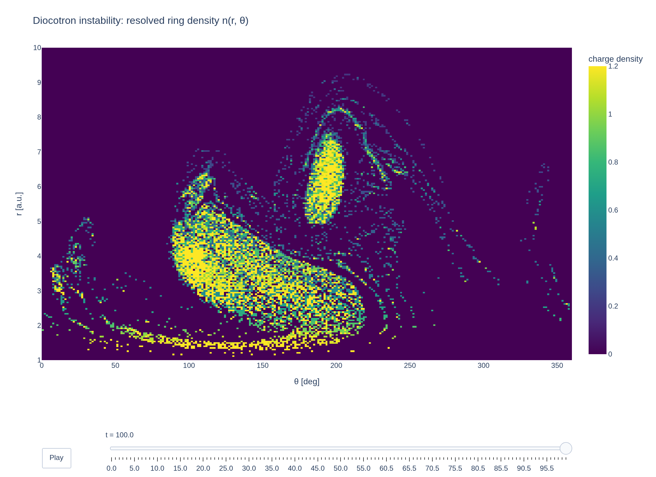
Loading interactive figure…
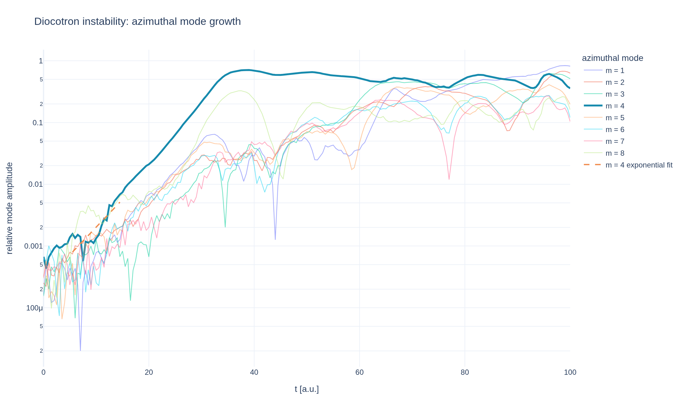
Loading interactive figure…
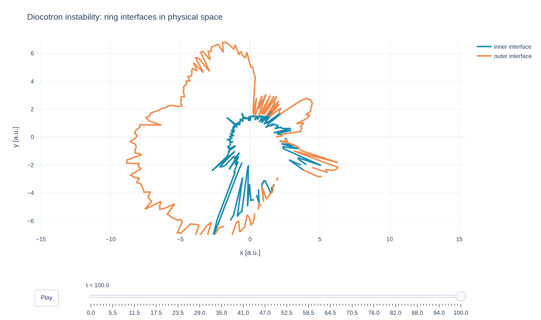
Physical problem
Shear instability in a rotating charged ring
PDEs solved by model:
Drift equation:
Poisson equation:
where is the guiding center distribution and
The control variate method can be activated in the Poisson equation; if enabled, the following Poisson equation is solved:
Simulation geometry
Domain used in this run
The actual HollowCylinder geometry reconstructed from this run's metadata. Switch between the 3D view and physical-coordinate slices.
Domain
HollowCylinder
Mapping
Loading HollowCylinder…
Parameters
| Parameter | Value | Description |
|---|---|---|
| Loading parameters… | ||
Performance
Profiling
Struphy's built-in scope-profiler instruments every propagator, pusher and solver call — these are the real per-call timings from the run above.
Durations
Gantt (rank 0)
Region statistics
| Region | Count | Avg (s) | Min (s) | Max (s) | Total (s) |
|---|
Complete source
Simulation script
Run it locally
1. Install and compile
Use Python 3.10 or newer with Struphy's system prerequisites installed. Run these commands in your Python environment:
pip install "struphy[pproc]>=3.4.0"
pip install "plasma-plots[plotly]>=0.1.1"
struphy compile
PNG exports need Chrome or Chromium. If Chrome is not installed, run kaleido_get_chrome.
2. Run the script
Download the .py file above, open a terminal in its directory, then run:
python diocotron-instability.pyFigures are saved in the current directory. Add --show to display them before saving.
"""Diocotron instability: a sheared E×B ring develops rippled edges.

An annular ring of charge, confined by a magnetic field, has a sheared E×B
rotation profile at its inner and outer edges. That shear is unstable: a
tiny azimuthal (mode number m) perturbation grows, rippling the ring's edges
-- the onset of the diocotron instability, a non-neutral-plasma analogue of
the Kelvin-Helmholtz instability, which given enough time rolls those
ripples up into a rotating pattern of discrete vortices.

Adapted from Struphy's maintained example
(examples/ToyGyrokinetic/diocotron_instability). Parameters follow Crouseilles,
Mehrenberger & Vecil (2014), https://doi.org/10.1140/epjd/e2014-50180-9.

Install dependencies and compile the kernels (Python 3.10 or newer):

    pip install "struphy[pproc]>=3.4.0"
    pip install "plasma-plots[plotly]>=0.1.1"
    struphy compile

PNG exports require Chrome or Chromium. If Chrome is not installed, run:

    kaleido_get_chrome

Save this file and run it from the directory where you want the output:

    python diocotron-instability.py

Figures are saved in the current directory; add --show to display them before saving.
"""

import argparse

import numpy as np
import plotly.graph_objects as go

from struphy import (
    BaseUnits,
    BinningPlot,
    BoundaryParameters,
    DerhamOptions,
    EnvironmentOptions,
    LoadingParameters,
    SavingParameters,
    Simulation,
    SortingParameters,
    Time,
    WeightsParameters,
    domains,
    equils,
    grids,
    maxwellians,
    perturbations,
)
from struphy.models import ToyDrift
from plasma_plots import save_figure

# A uniform-density ring between r = 4 and r = 5, seeded with a tiny m = 4 azimuthal mode.
r_minus, r_plus, mode_number = 4.0, 5.0, 4


def create_simulation() -> Simulation:
    model = ToyDrift(epsilon=1.0, alpha=1.0, base_units=BaseUnits(kBT=1.0))

    # An annular ring, r in [1, 10], with a uniform background field.
    domain = domains.HollowCylinder(a1=1.0, a2=10.0, Lz=10.0)
    equil = equils.HomogenSlab()
    grid = grids.TensorProductGrid(num_elements=(64, 64, 1), mpi_dims_mask=(False, True, False))
    derham_opts = DerhamOptions(degree=(3, 3, 1), bcs=(("dirichlet", "dirichlet"), None, None))
    time_opts = Time(dt=0.5, Tend=100.0, split_algo="LieTrotter")

    # A high-resolution radial-angular density snapshot at every step.  The extra
    # angular samples make the m = 4 ripples legible in the interactive movie.
    density_bins = BinningPlot(slice="e1_e2", n_bins=(192, 256), ranges=((0.0, 1.0), (0.0, 1.0)))
    model.kinetic_ions.set_markers(
        loading_params=LoadingParameters(ppc=40, loading="sobol_standard", spatial="disc"),
        weights_params=WeightsParameters(control_variate=True, reject_weights=True, threshold=0.0001),
        boundary_params=BoundaryParameters(),
        sorting_params=SortingParameters(boxes_per_dim=(16, 16, 1), do_sort=True, sorting_frequency=5),
        saving_params=SavingParameters(binning_plots=(density_bins,)),
        bufsize=2.0,
    )

    model.propagators.gc_poisson.options = model.propagators.gc_poisson.Options()
    model.propagators.push_gc_bxe.options = model.propagators.push_gc_bxe.Options(
        algo="discrete_gradient_1st_order_newton",
        evaluate_e_field=True,
    )
    a1, a2 = domain.params["a1"], domain.params["a2"]
    eta_minus, eta_plus = (r_minus - a1) / (a2 - a1), (r_plus - a1) / (a2 - a1)

    def ring_density(etas, r_minus=r_minus, r_plus=r_plus):
        radial = a1 + (a2 - a1) * etas[:, 0]
        return 1.0 * ((r_minus <= radial) & (radial < r_plus))

    model.kinetic_ions.var.add_background(maxwellians.GyroMaxwellian2D(n=(0.0, None)))
    perturbation = perturbations.ModesCos(amps=(1e-6,), ms=(mode_number,), perb_domain=((eta_minus, eta_plus), None, None))
    model.kinetic_ions.var.add_initial_condition(maxwellians.GyroMaxwellian2D(n=(ring_density, perturbation)))

    env = EnvironmentOptions(
        out_folders="struphy_gallery_runs",
        sim_folder="diocotron_instability",
    )
    sim = Simulation(
        model=model,
        name="Diocotron instability",
        description=(
            "A sheared E×B ring of charge is unstable: a tiny azimuthal "
            "perturbation grows, rippling the ring's edges — the onset of a "
            "rotating pattern of vortices."
            r" The charge ring starts from $$n(r,\theta,0)=\mathbf{1}_{[4,5)}(r)\,[1+10^{-6}\cos(4\theta)],$$"
            r" inside conducting cylinders at :math:`r=1` and :math:`r=10`; the indicator is one inside the ring and zero outside."
        ),
        env=env,
        time_opts=time_opts,
        domain=domain,
        equil=equil,
        grid=grid,
        derham_opts=derham_opts,
    )
    return sim


def pproc(sim: Simulation, show: bool = False):
    a1, a2 = sim.domain.params["a1"], sim.domain.params["a2"]

    output = sim.output.pproc(create_vtk=False)

    density = output.evaluate("kinetic_ions/e1_e2_density/f")
    radius = a1 + (a2 - a1) * np.asarray(density.eta1)
    angle_deg = 360.0 * np.asarray(density.eta2)
    frames_data = np.asarray(density)  # (time, radius, angle)
    times = np.asarray(density.t)

    # Resolve the azimuthal spectrum inside the initial ring.  This makes the
    # seeded m = 4 mode visible as a measurement rather than just a feature in
    # the animation.
    theta = np.deg2rad(angle_deg)
    ring = density.isel(eta1=(radius >= r_minus) & (radius <= r_plus))
    spectrum = abs(ring.plasma.analysis.mode_spectrum(dims="eta2", names="m").mean("eta1")) / ring.mean(("eta1", "eta2"))
    mode_amplitudes = {m: spectrum.sel(m=m) for m in range(1, 9)}
    growth_window = (times > 5.0) & (times < 15.0)
    growth_fit = mode_amplitudes[mode_number].isel(t=growth_window).plasma.analysis.growth_rate()
    growth_rate = growth_fit.rate
    print(f"Measured m = {mode_number} growth rate: {growth_rate:.4f}")

    # Keep the high-resolution movie responsive by using evenly spaced frames
    # instead of embedding all 1,250 saved timesteps.
    n_frames = min(120, len(frames_data))
    frame_indices = np.linspace(0, len(frames_data) - 1, n_frames, dtype=int)
    frames = [
        go.Frame(name=f"{times[idx]:.1f}", data=[go.Heatmap(z=frames_data[idx], x=angle_deg, y=radius, zmin=0, zmax=1.2, colorscale="Viridis")])
        for idx in frame_indices
    ]
    # Default to the final (most visibly rippled) frame -- both for the
    # interactive page's initial view and for the static PNG export, which
    # can only ever capture the base `data`, not the animation frames.
    figure = go.Figure(
        data=[go.Heatmap(z=frames_data[-1], x=angle_deg, y=radius, zmin=0, zmax=1.2, colorscale="Viridis", colorbar={"title": "charge density"})],
        frames=frames,
    )
    figure.update_layout(
        title="Diocotron instability: resolved ring density n(r, θ)",
        xaxis_title="θ [deg]",
        yaxis_title="r [a.u.]",
        template="plotly_white",
        autosize=True,
        margin={"l": 70, "r": 30, "t": 80, "b": 130},
        updatemenus=[
            {
                "type": "buttons",
                "showactive": False,
                "x": 0.0,
                "xanchor": "left",
                "y": -0.28,
                "yanchor": "top",
                "buttons": [
                    {
                        "label": "Play",
                        "method": "animate",
                        "args": [None, {"frame": {"duration": 30, "redraw": True}, "fromcurrent": True}],
                    },
                ],
            },
        ],
        sliders=[
            {
                "steps": [
                    {"args": [[frame.name], {"frame": {"duration": 0, "redraw": True}, "mode": "immediate"}], "label": frame.name, "method": "animate"}
                    for frame in frames
                ],
                "active": len(frames) - 1,
                "x": 0.12,
                "len": 0.88,
                "y": -0.18,
                "currentvalue": {"prefix": "t = "},
            },
        ],
    )

    save_figure(figure, "diocotron-instability", height=800, show=show)

    mode_figure = go.Figure()
    for m, amplitude in mode_amplitudes.items():
        mode_figure.add_trace(go.Scatter(
            x=times,
            y=amplitude.values + 1e-12,
            mode="lines",
            name=f"m = {m}",
            line={"width": 3 if m == mode_number else 1.2, "color": "#168aad" if m == mode_number else None},
            opacity=1.0 if m == mode_number else 0.55,
        ))
    mode_figure.add_trace(go.Scatter(
        x=growth_fit.time,
        y=growth_fit.fitted,
        mode="lines",
        name=f"m = {mode_number} exponential fit",
        line={"dash": "dash", "color": "#f08a4b", "width": 2},
    ))
    mode_figure.update_layout(
        title="Diocotron instability: azimuthal mode growth",
        xaxis_title="t [a.u.]",
        yaxis_title="relative mode amplitude",
        yaxis={"type": "log"},
        template="plotly_white",
        margin={"l": 70, "r": 30, "t": 80, "b": 60},
        legend={"title": "azimuthal mode"},
    )

    # The same density data viewed in physical x-y coordinates.  Plotting the
    # inner and outer density interfaces makes the rotating four-lobed shape
    # immediately recognizable, unlike a rectangular r-theta heatmap.
    interface_level = 0.2

    def interface_traces(frame):
        occupied = frame >= interface_level
        inner, outer = [], []
        for column in occupied.T:
            indices = np.flatnonzero(column)
            inner.append(radius[indices[0]] if len(indices) else np.nan)
            outer.append(radius[indices[-1]] if len(indices) else np.nan)

        def curve(values, name, color):
            values = np.asarray(values)
            closed_r = np.append(values, values[0])
            closed_theta = np.append(theta, theta[0])
            return go.Scatter(
                x=closed_r * np.cos(closed_theta),
                y=closed_r * np.sin(closed_theta),
                mode="lines",
                name=name,
                line={"color": color, "width": 3},
                connectgaps=False,
            )

        return [curve(inner, "inner interface", "#168aad"), curve(outer, "outer interface", "#f08a4b")]

    interface_frames = [go.Frame(name=f"{times[idx]:.1f}", data=interface_traces(frames_data[idx])) for idx in frame_indices]
    interface_figure = go.Figure(data=interface_traces(frames_data[-1]), frames=interface_frames)
    interface_figure.update_layout(
        title="Diocotron instability: ring interfaces in physical space",
        xaxis={"title": "x [a.u.]", "range": [-7, 7], "scaleanchor": "y", "scaleratio": 1},
        yaxis={"title": "y [a.u.]", "range": [-7, 7]},
        template="plotly_white",
        margin={"l": 70, "r": 30, "t": 80, "b": 130},
        updatemenus=[{"type": "buttons", "showactive": False, "x": 0.0, "xanchor": "left", "y": -0.28, "yanchor": "top", "buttons": [{"label": "Play", "method": "animate", "args": [None, {"frame": {"duration": 45, "redraw": True}, "fromcurrent": True}]}]}],
        sliders=[{"steps": [{"args": [[frame.name], {"frame": {"duration": 0, "redraw": True}, "mode": "immediate"}], "label": frame.name, "method": "animate"} for frame in interface_frames], "active": len(interface_frames) - 1, "x": 0.12, "len": 0.88, "y": -0.18, "currentvalue": {"prefix": "t = "}}],
    )

    save_figure(mode_figure, "diocotron-instability-mode-growth", show=show)
    save_figure(interface_figure, "diocotron-instability-ring-interfaces", show=show)


if __name__ == "__main__":
    argparser = argparse.ArgumentParser(description="Run the diocotron instability example.")
    argparser.add_argument(
        "--pproc-only",
        action="store_true",
        help="Run post-processing on an existing simulation instead of running a new one.",
    )
    argparser.add_argument("--show", action="store_true", help="Show the figures before saving them.")
    args = argparser.parse_args()

    simulation = create_simulation()
    if not args.pproc_only:
        simulation.run()
    pproc(simulation, show=args.show)
See the post-processing guide for more ways to inspect the result.