Gas expansion into vacuum

An isothermal gas initially occupies the left part of a one-dimensional box and expands into the vacuum. Smoothed particle hydrodynamics follows the rarefaction wave and the gas streaming into the vacuum, and the result is compared with the exact self-similar solution.

← All examples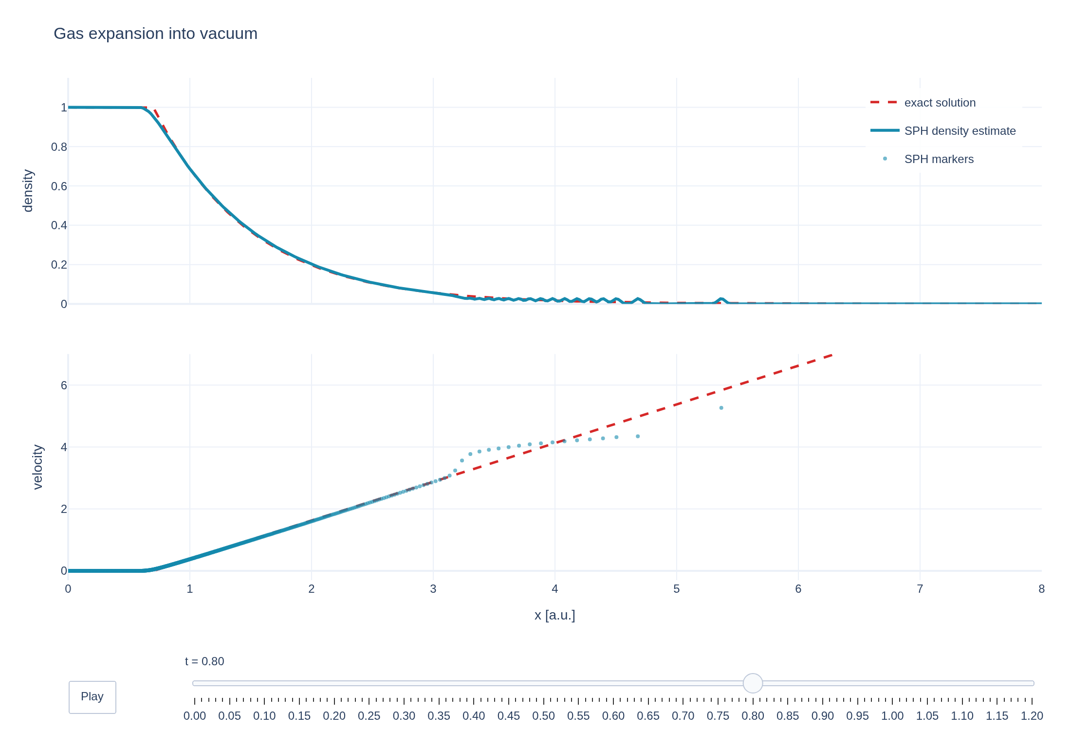

Actual output from the script below: the SPH density estimate (top) and the velocities of the 768 markers (bottom), with the exact solution dashed. Press Play or drag the slider; the still image shows t = 0.8. The density stays within 1.9% of the exact solution on average (relative L1 error) and within 2.5% at the end of the run. In the thin tail, where the density is below about 0.05, only a few markers are left; they move more slowly than the exact solution.

The 768 SPH particles move from the initially filled region into the vacuum; color shows velocity. The dashed line marks the initial gas edge. Vertical lanes only separate the particles visually: this simulation is one-dimensional. Press Play, Pause, or drag the time slider.

The density (top) and the marker velocities (bottom) at four times against the similarity variable (x − x₀) / t, with the exact solution dashed. From ξ = −1, where the rarefaction starts, up to ξ ≈ 2 the four times fall on one curve. The earliest time is smoothed around ξ = −1 because the release is smoothed over the kernel width. Beyond ξ ≈ 2, where the density is below about 0.05, only a few markers are left: they move more slowly than the exact solution and their density estimate is noisy.

The error of the SPH result against the exact solution for t ≥ 0.1. The density error, the L1 difference relative to the exact density, stays between 1.3% and 2.5%. The rms error of the marker velocity grows to 7.7% of the sound speed, but the median marker is off by only 0.9% at the end: the rms is dominated by the few fast markers in the low-density tail.

Physical problem

A gas released into vacuum

An isothermal gas of density 1 fills the part x < 1.5 of a one-dimensional box of length 8, at rest, and the rest of the box is empty. When the gas is released, a rarefaction wave runs into it at the sound speed c = 1 while the gas streams into the vacuum. The tutorial this example is adapted from expands a two-dimensional Gaussian blob, which has no simple exact solution; the half-box release reduces the problem to one dimension.

For the isothermal pressure p = κρ, the sound speed is c = √κ and the flow depends only on ξ = (x − x₀)/t. The gas is undisturbed for ξ < −c. Beyond that, the Riemann invariant u + c ln ρ is constant and the characteristics give u = ξ + c and ρ = ρ₀ exp(−(ξ/c + 1)). The density decays exponentially and never reaches zero, so the gas has no sharp front, and the velocity grows without bound with ξ. The SPH run uses no viscosity, and the box is long enough that no marker reaches the right wall during the run. The density estimate conserves the mass to 2e-5 (relative).

PDEs solved by model:

Continuity:

\partial_{t} ρ + \nabla \cdot (ρ u) = 0

Momentum:

ρ (\partial_{t} u + u \cdot \nabla u) = - \nabla (ρ^{2} \frac{\partial U ( ρ , S )}{\partial ρ}) - \nabla \cdot π

Entropy:

\partial_{t} S + u \cdot \nabla S = 0

where $S$ denotes the entropy per unit mass and $π$ is the viscous stress tensor.

The viscous stress tensor for a Newtonian fluid is given by:

σ = - μ (\nabla u + (\nabla u)^{T} - \frac{2}{3} (\nabla \cdot u) I)

where $μ$ is the dynamic (shear) viscosity and $I$ is the identity tensor.

The internal energy per unit mass can be defined in two ways:

isothermal : U (ρ, S) = κ (S) lo g ρ

polytropic : U (ρ, S) = κ (S) \frac{ρ ^{γ - 1}}{γ - 1}

Model: ViscousEulerSPH
Domain: Cuboid (r1=8)
Markers: 768
SPH kernel: Gaussian, 1D
Sound speed: 1
Integrator: Forward euler
Evolution: 120 steps
Visualization: Plotly

Performance

Profiling

Download profile .h5

Struphy's built-in scope-profiler instruments every propagator, pusher and solver call — these are the real per-call timings from the run above, rendered live from its data.

Durations

Gantt (rank 0)

Region statistics

Region	Count	Avg (s)	Min (s)	Max (s)	Total (s)

Complete source

Run the simulation

Download .py

Requires Struphy 3.2 with compiled kernels and Plotly. Run struphy compile once, then execute python gas-expansion.py.

"""Gas expansion into vacuum: an isothermal gas released from a half box.

A uniform isothermal gas fills the left part of a one-dimensional box, and the rest is empty. When the
gas is released, a rarefaction wave travels into it at the sound speed while the gas streams into the
vacuum. The flow has a known self-similar solution, to which the smoothed particle hydrodynamics (SPH)
result can be compared.

Adapted from Struphy's tutorial (tutorials/tutorial_gas_expansion_sph.ipynb), reduced to one dimension
so that an exact solution exists.

Requires Struphy 3.2 with compiled kernels (`struphy compile`).
"""

import numpy as np
import plotly.graph_objects as go

from struphy import (
    BoundaryParameters,
    EnvironmentOptions,
    KernelDensityPlot,
    LoadingParameters,
    SavingParameters,
    Simulation,
    SortingParameters,
    Time,
    WeightsParameters,
    domains,
    equils,
)
from struphy.models import ViscousEulerSPH
from struphy.ode.utils import ButcherTableau

# The gas is isothermal, p = kappa * rho, so the sound speed is c = sqrt(kappa) = 1.
kappa = 1.0
sound_speed = np.sqrt(kappa)
gas_density = 1.0
box_length = 8.0
release_point = 1.5  # the gas fills x < release_point at t = 0
boxes = 64
markers_per_box = 64
density_points = 401

model = ViscousEulerSPH(with_B0=False, with_p=True, with_viscosity=False)
model.propagators.push_eta.options = model.propagators.push_eta.Options(
    butcher=ButcherTableau(algo="forward_euler"),
)
model.propagators.push_sph_p.options = model.propagators.push_sph_p.Options(kernel_type="gaussian_1d", kappa=kappa)

domain = domains.Cuboid(r1=box_length)
model.euler_fluid.set_markers(
    loading_params=LoadingParameters(ppb=markers_per_box, loading="tesselation"),
    # Markers are loaded over the whole box, and those with almost no weight (the vacuum) are removed.
    weights_params=WeightsParameters(reject_weights=True, threshold=1e-6),
    boundary_params=BoundaryParameters(
        bc=("reflect", "periodic", "periodic"), bc_sph=("mirror", "periodic", "periodic")
    ),
    sorting_params=SortingParameters(boxes_per_dim=(boxes, 1, 1), dims_mask=(True, False, False)),
    saving_params=SavingParameters(
        n_markers=1.0,
        kernel_density_plots=(KernelDensityPlot(pts_e1=density_points, pts_e2=1),),
    ),
    bufsize=2,
)
model.euler_fluid.var.add_background(
    equils.ConstantVelocity(density_profile="step_function_xy", n=gas_density, upper_x=release_point),
)

env = EnvironmentOptions(
    out_folders="struphy_gallery_runs",
    sim_folder="gas_expansion",
)
sim = Simulation(
    model=model,
    name="Gas expansion into vacuum",
    description=(
        "An isothermal gas initially occupies the left part of a one-dimensional box and expands into "
        "the vacuum. Smoothed particle hydrodynamics follows the rarefaction wave "
        "and the gas streaming into the vacuum, and the result is compared with the "
        "exact self-similar solution."
    ),
    env=env,
    time_opts=Time(dt=0.01, Tend=1.2, split_algo="Strang"),
    domain=domain,
    grid=None,
    derham_opts=None,
)


def exact_solution(positions, time):
    """The exact isothermal rarefaction into vacuum: density and velocity at `time`.

    Gas of density `gas_density` at rest fills x < `release_point` at t = 0. For xi = (x - x0) / t below
    -c the gas is undisturbed. Above, the Riemann invariant u + c ln(rho) = c ln(rho_0) and the
    self-similar characteristic u = xi + c give rho = rho_0 exp(-(xi / c + 1)) and u = xi + c.
    """
    if time <= 0.0:
        return np.where(positions < release_point, gas_density, 0.0), np.zeros_like(positions)
    xi = (positions - release_point) / time
    undisturbed = xi < -sound_speed
    density = np.where(undisturbed, gas_density, gas_density * np.exp(-(xi / sound_speed + 1.0)))
    velocity = np.where(undisturbed, 0.0, xi + sound_speed)
    return density, velocity


if __name__ == "__main__":
    from plotly.subplots import make_subplots

    from _gallery import export_profiling, merge_metadata, publish_thumbnail, save_extra_figure, save_figure

    output = sim.run(profiling_activated=True)
    output.pproc()

    density = output.evaluate("euler_fluid/view_0/n").isel(e2=0, e3=0)  # (t, e1): the SPH density estimate
    orbits = output.evaluate("euler_fluid")  # (t, marker, quantity)
    times = orbits.t.values
    assert np.allclose(times, density.t.values)
    grid = density.e1.values * box_length
    marker_position = orbits.sel(quantity="x").values  # (t, marker)
    marker_velocity = orbits.sel(quantity="v1").values

    # How far the SPH result is from the exact solution, on the density grid inside the box and on the
    # velocities of all markers. The exact solution is singular at t = 0, so only t >= 0.1 is compared.
    window = (grid > 0.05) & (grid < box_length - 0.5)

    def density_error(index):
        exact_density, _ = exact_solution(grid, times[index])
        difference = np.abs(density.isel(t=index).values - exact_density)
        return np.trapezoid(difference[window], grid[window]) / np.trapezoid(exact_density[window], grid[window])

    def velocity_error(index):
        _, exact_velocity = exact_solution(marker_position[index], times[index])
        return np.sqrt(np.mean((marker_velocity[index] - exact_velocity) ** 2)) / sound_speed

    def velocity_median_error(index):
        _, exact_velocity = exact_solution(marker_position[index], times[index])
        return np.median(np.abs(marker_velocity[index] - exact_velocity)) / sound_speed

    compared = np.flatnonzero(times >= 0.1)
    density_errors = np.array([density_error(i) for i in compared])
    velocity_errors = np.array([velocity_error(i) for i in compared])
    velocity_median_final = float(velocity_median_error(compared[-1]))
    mass = np.array([np.trapezoid(density.isel(t=i).values, grid) for i in range(len(times))])
    mass_error = float(np.max(np.abs(mass / (gas_density * release_point) - 1.0)))
    print(
        f"Density error (relative L1): mean {density_errors.mean():.4f}, final {density_errors[-1]:.4f}; "
        f"velocity error (rms, units of c): mean {velocity_errors.mean():.4f}, final {velocity_errors[-1]:.4f}, "
        f"median final {velocity_median_final:.4f}; "
        f"mass error {mass_error:.1e}"
    )

    # The animation: density (top) and marker velocities (bottom) against the exact solution.
    profile_grid = np.linspace(0.0, box_length, 800)

    def frame_traces(index, webgl=False):
        exact_density, exact_velocity = exact_solution(profile_grid, times[index])
        markers = go.Scattergl if webgl else go.Scatter
        exact_style = {"color": "#d62828", "width": 2.5, "dash": "dash"}
        return [
            go.Scatter(
                x=profile_grid,
                y=exact_density,
                mode="lines",
                name="exact solution",
                line=exact_style,
                legendgroup="exact",
                xaxis="x",
                yaxis="y",
            ),
            go.Scatter(
                x=grid,
                y=density.isel(t=index).values,
                mode="lines",
                name="SPH density estimate",
                line={"color": "#168aad", "width": 3},
                xaxis="x",
                yaxis="y",
            ),
            go.Scatter(
                x=profile_grid,
                y=exact_velocity,
                mode="lines",
                name="exact solution",
                line=exact_style,
                legendgroup="exact",
                showlegend=False,
                xaxis="x2",
                yaxis="y2",
            ),
            markers(
                x=marker_position[index],
                y=marker_velocity[index],
                mode="markers",
                name="SPH markers",
                marker={"size": 4, "color": "#168aad", "opacity": 0.6},
                xaxis="x2",
                yaxis="y2",
            ),
        ]

    figure = make_subplots(rows=2, cols=1, shared_xaxes=True, vertical_spacing=0.1)
    for row, trace_group in ((1, (0, 1)), (2, (2, 3))):
        for trace in (frame_traces(0)[i] for i in trace_group):
            figure.add_trace(trace, row=row, col=1)
    frames = [go.Frame(name=f"{times[i]:.2f}", data=frame_traces(i), traces=[0, 1, 2, 3]) for i in range(len(times))]
    figure.frames = frames
    figure.update_xaxes(range=[0, box_length], row=2, col=1, title_text="x [a.u.]")
    figure.update_yaxes(range=[0, 1.15], row=1, col=1, title_text="density")
    figure.update_yaxes(range=[-0.3, 7.0], row=2, col=1, title_text="velocity")
    figure.update_layout(
        title="Gas expansion into vacuum",
        template="plotly_white",
        autosize=True,
        legend={"x": 0.98, "y": 0.98, "xanchor": "right", "bgcolor": "rgba(255,255,255,0.82)"},
        margin={"l": 70, "r": 30, "t": 80, "b": 130},
        updatemenus=[
            {
                "type": "buttons",
                "showactive": False,
                "x": 0.0,
                "xanchor": "left",
                "y": -0.2,
                "yanchor": "top",
                "buttons": [
                    {
                        "label": "Play",
                        "method": "animate",
                        "args": [None, {"frame": {"duration": 40, "redraw": True}, "fromcurrent": True}],
                    },
                ],
            },
        ],
        sliders=[
            {
                "steps": [
                    {
                        "args": [[frame.name], {"frame": {"duration": 0, "redraw": True}, "mode": "immediate"}],
                        "label": frame.name,
                        "method": "animate",
                    }
                    for frame in frames
                ],
                "active": 0,
                "x": 0.12,
                "len": 0.88,
                "y": -0.1,
                "currentvalue": {"prefix": "t = "},
            },
        ],
    )
    still_index = int(np.argmin(np.abs(times - 0.8)))
    save_figure(
        figure,
        "gas-expansion",
        height=750,
        static_data=frame_traces(still_index, webgl=False),
        static_active=still_index,
    )

    # A spatial view of every SPH particle. Fixed display lanes separate overlapping particles;
    # only x is a physical coordinate in this one-dimensional simulation.
    particle_lanes = (np.arange(marker_position.shape[1]) % 16 + 0.5) / 16

    def particle_trace(index):
        return go.Scatter(
            x=marker_position[index],
            y=particle_lanes,
            mode="markers",
            marker={
                "size": 5,
                "color": marker_velocity[index],
                "colorscale": "Viridis",
                "cmin": 0,
                "cmax": float(np.max(marker_velocity)),
                "colorbar": {"title": "velocity"},
            },
            customdata=marker_velocity[index],
            hovertemplate="x = %{x:.3f}<br>velocity = %{customdata:.3f}<extra>SPH particle</extra>",
            showlegend=False,
        )

    particles = go.Figure(data=[particle_trace(0)])
    particles.frames = [
        go.Frame(name=f"{time:.2f}", data=[particle_trace(i)], traces=[0])
        for i, time in enumerate(times)
    ]
    particles.update_layout(
        title="Gas expansion: SPH particles",
        template="plotly_white",
        autosize=True,
        xaxis={"title": "x [a.u.]", "range": [0, box_length]},
        yaxis={"range": [0, 1], "visible": False, "fixedrange": True},
        margin={"l": 55, "r": 100, "t": 85, "b": 130},
        updatemenus=[{
            "type": "buttons", "direction": "left", "showactive": False,
            "x": 0, "xanchor": "left", "y": -0.23, "yanchor": "top",
            "buttons": [
                {"label": "Play", "method": "animate", "args": [None, {
                    "frame": {"duration": 60, "redraw": True},
                    "transition": {"duration": 0}, "fromcurrent": True,
                }]},
                {"label": "Pause", "method": "animate", "args": [[None], {
                    "mode": "immediate", "frame": {"duration": 0, "redraw": False},
                    "transition": {"duration": 0},
                }]},
            ],
        }],
        sliders=[{
            "active": 0, "x": 0, "len": 1, "y": -0.08,
            "currentvalue": {"prefix": "t = "},
            "steps": [{
                "label": frame.name, "method": "animate",
                "args": [[frame.name], {"mode": "immediate",
                    "frame": {"duration": 0, "redraw": True}, "transition": {"duration": 0}}],
            } for frame in particles.frames],
        }],
    )
    particles.add_vline(x=release_point, line_dash="dash", line_color="#64748b",
                        annotation_text="initial gas edge", annotation_position="top right")
    particle_figure = save_extra_figure(
        particles, "gas-expansion", "particles",
        alt="Animation of SPH particles expanding into vacuum, colored by velocity",
        caption=(
            "The 768 SPH particles move from the initially filled region into the vacuum; color shows velocity. "
            "The dashed line marks the initial gas edge. Vertical lanes only separate the particles visually: "
            "this simulation is one-dimensional. Press Play, Pause, or drag the time slider."
        ),
    )

    # The same data against the similarity variable xi = (x - x0) / t, where every time falls on one curve.
    similarity = make_subplots(rows=2, cols=1, shared_xaxes=True, vertical_spacing=0.1)
    xi_line = np.linspace(-2.5, 5.0, 600)
    exact_density_line, exact_velocity_line = exact_solution(release_point + xi_line, 1.0)
    similarity.add_scatter(
        x=xi_line,
        y=exact_density_line,
        mode="lines",
        name="exact solution",
        line={"color": "black", "width": 2.5, "dash": "dash"},
        legendgroup="exact",
        row=1,
        col=1,
    )
    similarity.add_scatter(
        x=xi_line,
        y=exact_velocity_line,
        mode="lines",
        name="exact solution",
        line={"color": "black", "width": 2.5, "dash": "dash"},
        legendgroup="exact",
        showlegend=False,
        row=2,
        col=1,
    )
    for target, color in zip((0.2, 0.4, 0.8, 1.2), ("#f77f00", "#d62828", "#7b2cbf", "#168aad")):
        index = int(np.argmin(np.abs(times - target)))
        xi_grid = (grid - release_point) / times[index]
        similarity.add_scatter(
            x=xi_grid,
            y=density.isel(t=index).values,
            mode="lines",
            name=f"SPH, t = {times[index]:.1f}",
            line={"color": color, "width": 2.5},
            legendgroup=f"t{index}",
            row=1,
            col=1,
        )
        similarity.add_scatter(
            x=(marker_position[index] - release_point) / times[index],
            y=marker_velocity[index],
            mode="markers",
            marker={"size": 4, "color": color, "opacity": 0.6},
            legendgroup=f"t{index}",
            showlegend=False,
            row=2,
            col=1,
        )
    similarity.update_xaxes(range=[-2.5, 5.0], row=2, col=1, title_text="(x − x₀) / t")
    similarity.update_yaxes(title_text="density", row=1, col=1)
    similarity.update_yaxes(title_text="velocity", range=[-0.3, 6.5], row=2, col=1)
    similarity.update_layout(
        title="Gas expansion: all times fall on one self-similar curve",
        template="plotly_white",
        autosize=True,
        legend={"x": 0.98, "y": 0.98, "xanchor": "right", "bgcolor": "rgba(255,255,255,0.82)"},
        margin={"l": 70, "r": 30, "t": 80, "b": 60},
    )

    # The error against time.
    error_figure = go.Figure()
    error_figure.add_scatter(
        x=times[compared],
        y=100 * density_errors,
        mode="lines",
        name="density (relative L1 error, %)",
        line={"color": "#168aad", "width": 3},
    )
    error_figure.add_scatter(
        x=times[compared],
        y=100 * velocity_errors,
        mode="lines",
        name="marker velocity (rms error, % of c)",
        line={"color": "#d62828", "width": 3},
    )
    error_figure.update_layout(
        title="Gas expansion: error against the exact solution",
        xaxis_title="t [a.u.]",
        yaxis_title="error [%]",
        yaxis={"rangemode": "tozero"},
        template="plotly_white",
        autosize=True,
        legend={"x": 0.02, "y": 0.98, "bgcolor": "rgba(255,255,255,0.82)"},
        margin={"l": 70, "r": 30, "t": 80, "b": 60},
    )

    figures = [
        particle_figure,
        save_extra_figure(
            similarity,
            "gas-expansion",
            "similarity",
            alt="Density and velocity against the similarity variable at four times, on the exact curve",
            caption=(
                "The density (top) and the marker velocities (bottom) at four times against the similarity variable "
                "(x − x₀) / t, with the exact solution dashed. From ξ = −1, where the rarefaction starts, up to "
                "ξ ≈ 2 the four times fall on one curve. The earliest time is smoothed around ξ = −1 because the "
                "release is smoothed over the kernel width. Beyond ξ ≈ 2, where the density is below about 0.05, only "
                "a few markers are left: they move more slowly than the exact solution and their density estimate is "
                "noisy."
            ),
        ),
        save_extra_figure(
            error_figure,
            "gas-expansion",
            "error",
            alt="Density and velocity error of the SPH result against time",
            caption=(
                f"The error of the SPH result against the exact solution for t ≥ 0.1. The density error, the L1 "
                f"difference relative to the exact density, stays between {100 * density_errors.min():.1f}% and "
                f"{100 * density_errors.max():.1f}%. The rms error of the marker velocity grows to "
                f"{100 * velocity_errors[-1]:.1f}% of the sound speed, but the median marker is off by only "
                f"{100 * velocity_median_final:.1f}% at the end: the rms is dominated by the few fast markers in the "
                "low-density tail."
            ),
        ),
    ]

    profiling = export_profiling(sim, "gas-expansion")

    merge_metadata(
        "gas-expansion",
        soundSpeed=sound_speed,
        releasePoint=release_point,
        boxLength=box_length,
        markers=int(marker_position.shape[1]),
        kernel="Gaussian, 1D",
        densityErrorMean=float(density_errors.mean()),
        densityErrorFinal=float(density_errors[-1]),
        velocityErrorMean=float(velocity_errors.mean()),
        velocityErrorFinal=float(velocity_errors[-1]),
        velocityMedianErrorFinal=velocity_median_final,
        massError=mass_error,
        figures=figures,
        **publish_thumbnail("gas-expansion"),
        **profiling,
    )

Adapted from Struphy’s gas-expansion SPH tutorial, reduced to one dimension so that an exact solution exists. See the post-processing guide for more ways to inspect the result.