DriftKineticElectrostaticAdiabatic · Drift-kinetic turbulence
ITG drift wave
A magnetized plasma column with radial density and temperature gradients drives a helical drift wave unstable — the basic mechanism behind ion-temperature-gradient (ITG) turbulence. The initial helical density seed is with . The background temperature is .
Loading interactive figure…
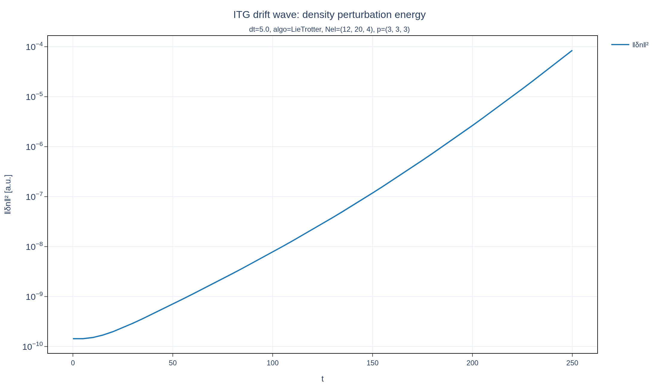
Loading interactive figure…
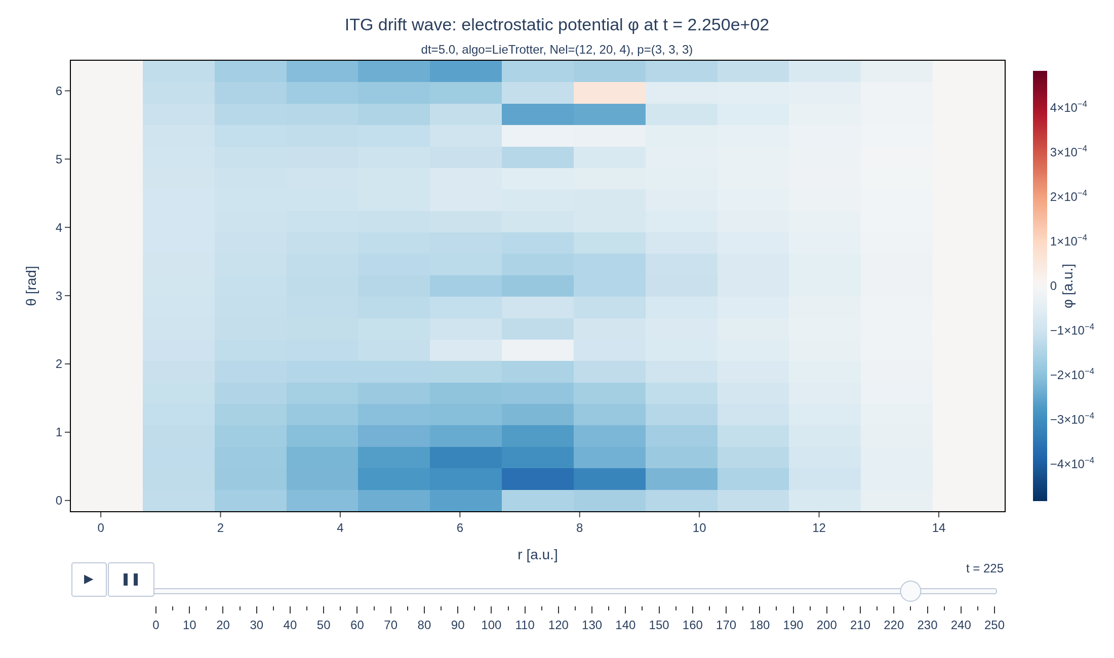
Loading interactive figure…
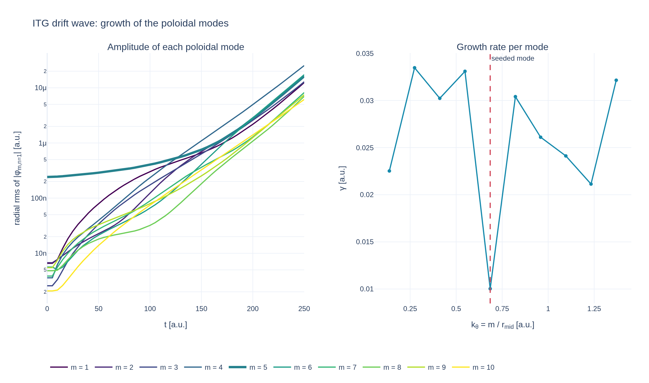
Loading interactive figure…
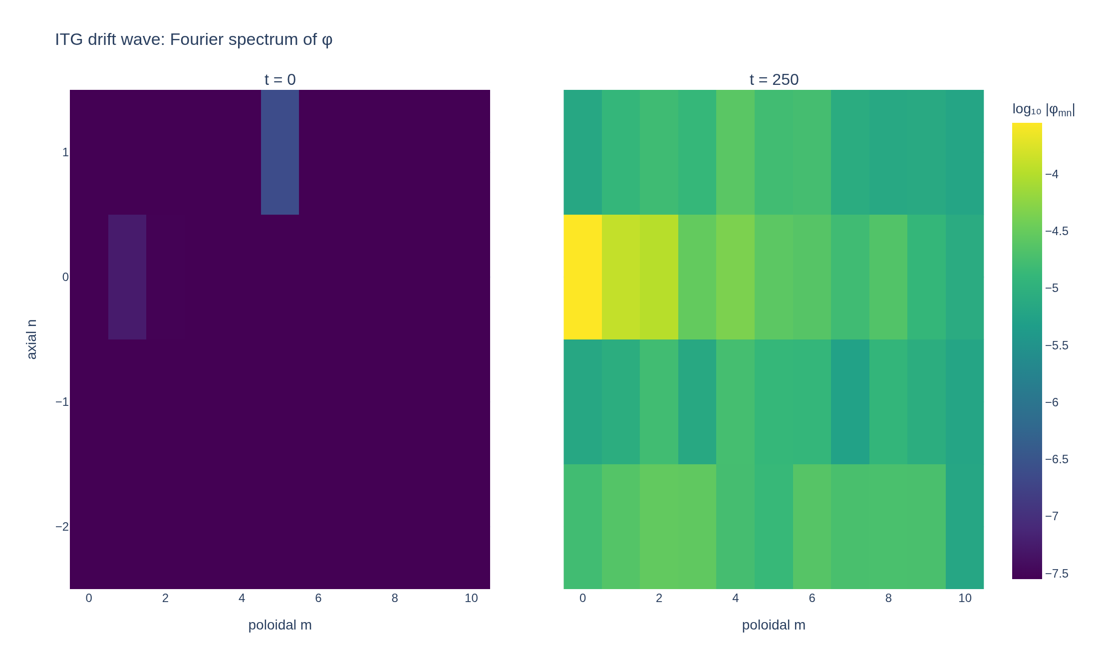
Loading interactive figure…
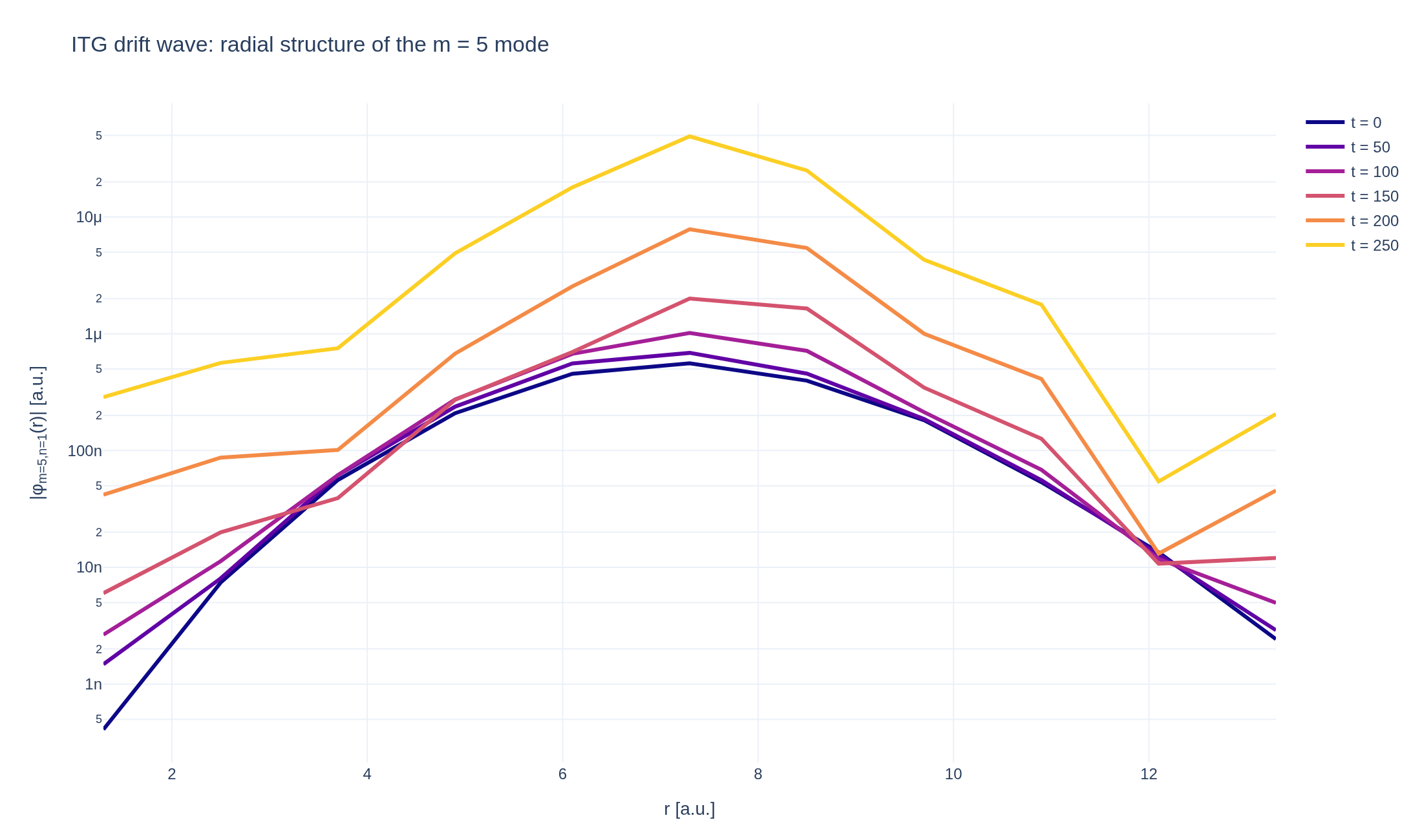
Loading interactive figure…
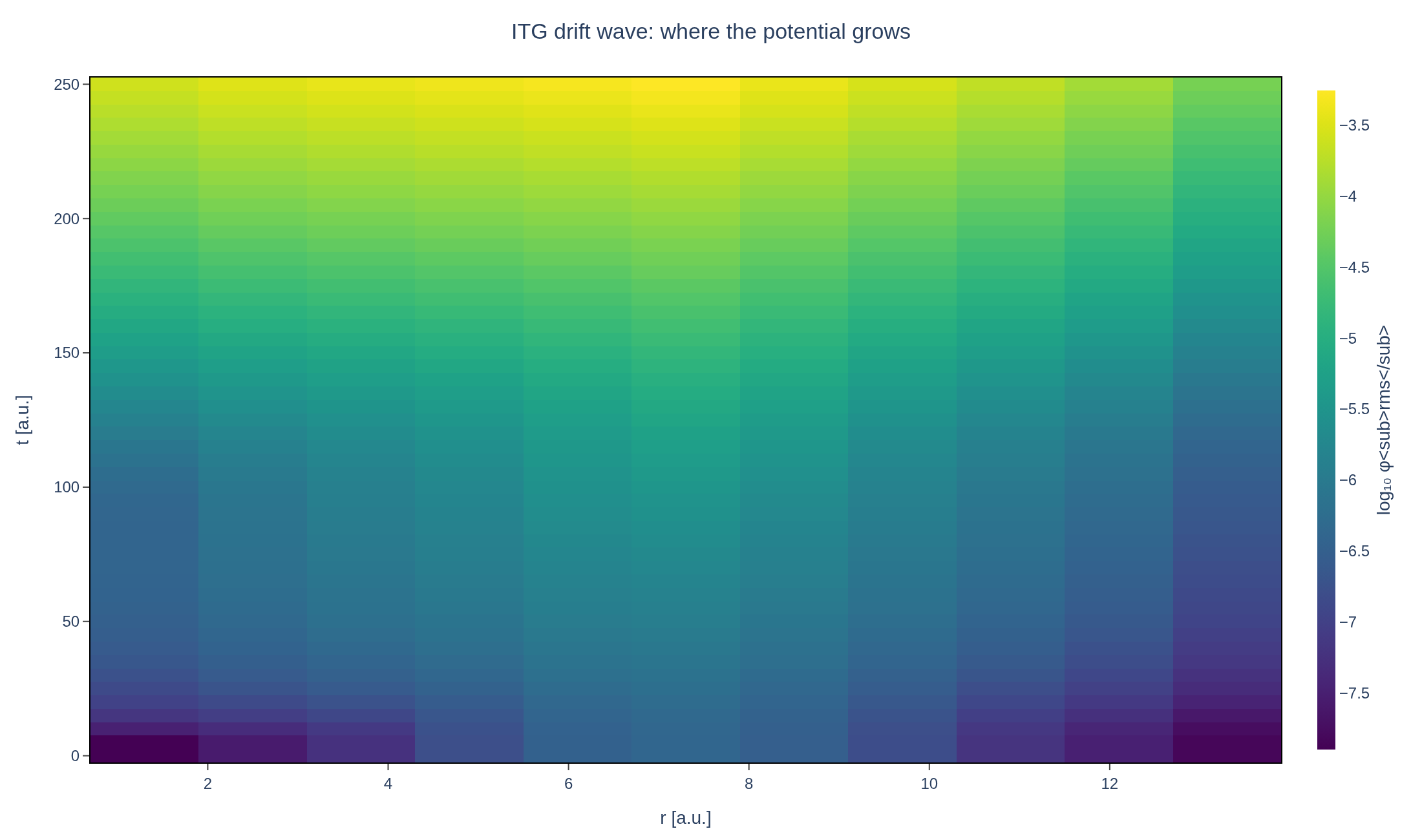
Loading interactive figure…
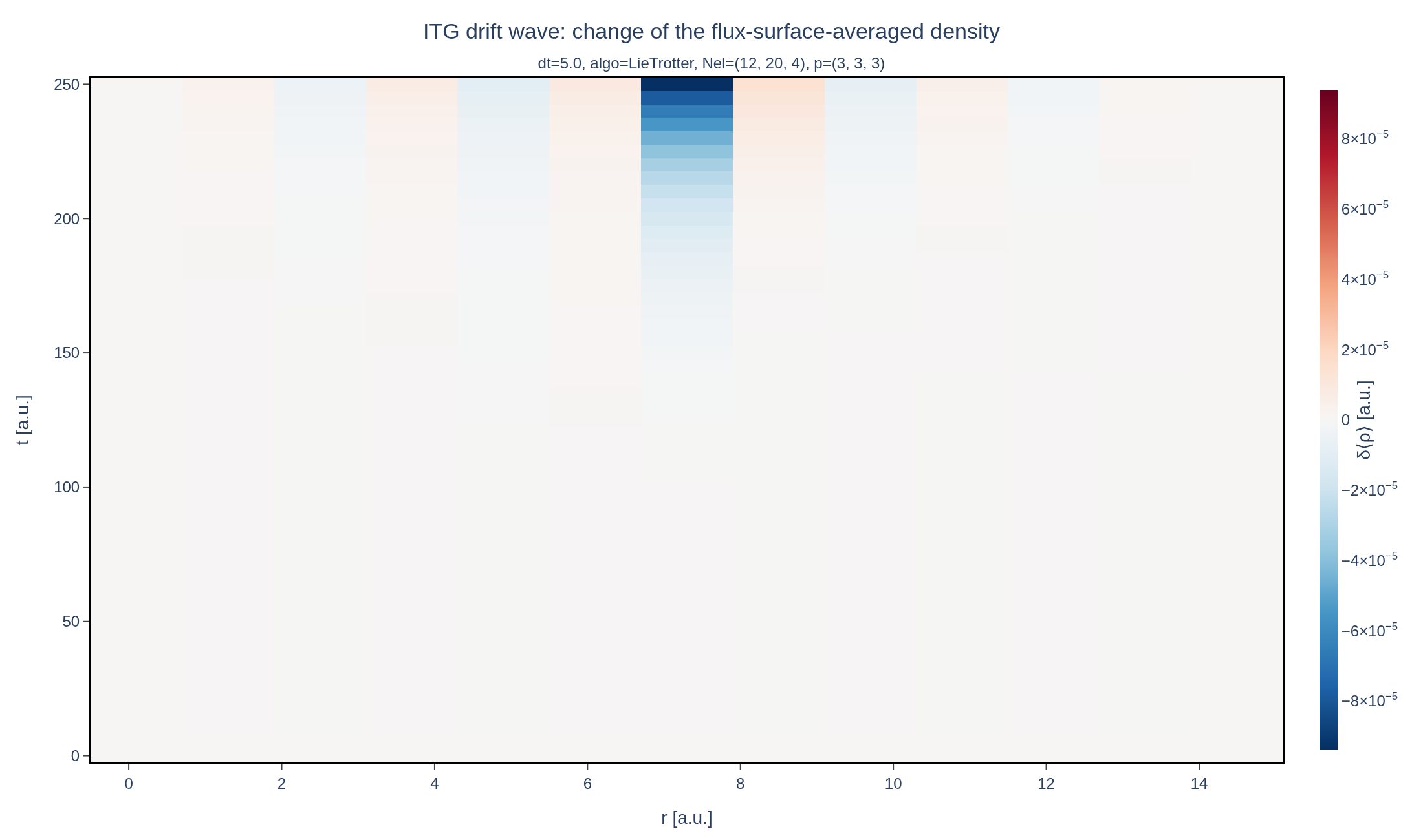
Physical problem
Drift waves from a temperature gradient
PDEs solved by model:
Drift-kinetic equation:
Poisson equation:
where is the guiding center distribution and
The control variate method can be activated in the Poisson equation; if enabled, the following Poisson equation is solved:
Simulation geometry
Domain used in this run
The actual HollowCylinder geometry reconstructed from this run's metadata. Switch between the 3D view and physical-coordinate slices.
Domain
HollowCylinder
Mapping
Loading HollowCylinder…
Parameters
| Parameter | Value | Description |
|---|---|---|
| Loading parameters… | ||
Performance
Profiling
Struphy's built-in scope-profiler instruments every propagator, pusher and solver call — these are the real per-call timings from the run above.
Durations
Gantt (rank 0)
Region statistics
| Region | Count | Avg (s) | Min (s) | Max (s) | Total (s) |
|---|
Complete source
Simulation script
Run it locally
1. Install and compile
Use Python 3.10 or newer with Struphy's system prerequisites installed. Run these commands in your Python environment:
pip install "struphy[pproc]>=3.4.0"
pip install "plasma-plots[plotly]>=0.1.1"
struphy compile
PNG exports need Chrome or Chromium. If Chrome is not installed, run kaleido_get_chrome.
2. Run the script
Download the .py file above, open a terminal in its directory, then run:
python itg-drift-wave.pyFigures are saved in the current directory. Add --show to display them before saving.
"""ITG drift wave: a temperature-gradient-driven instability in a cylinder.

A magnetized plasma column with radial density and temperature gradients is
unstable to drift waves: a small helical density perturbation taps the free
energy in the ion-temperature gradient (ITG) and grows exponentially,
extracting energy from the background profiles -- the basic mechanism behind
ITG turbulence, one of the dominant sources of turbulent transport in
magnetically confined fusion plasmas.

Adapted from Struphy's maintained example
(examples/DriftKineticElectrostaticAdiabatic/itg_cylindre), at reduced
resolution and run length to keep it a quick gallery run.

Install dependencies and compile the kernels (Python 3.10 or newer):

    pip install "struphy[pproc]>=3.4.0"
    pip install "plasma-plots[plotly]>=0.1.1"
    struphy compile

PNG exports require Chrome or Chromium. If Chrome is not installed, run:

    kaleido_get_chrome

Save this file and run it from the directory where you want the output:

    python itg-drift-wave.py

Figures are saved in the current directory; add --show to display them before saving.
"""

import argparse

import numpy as np
import plotly.graph_objects as go
import xarray as xr
from plotly.colors import sample_colorscale

from struphy import (
    BaseUnits,
    BinningPlot,
    BoundaryParameters,
    DerhamOptions,
    EnvironmentOptions,
    LoadingParameters,
    SavingParameters,
    Simulation,
    SortingParameters,
    Time,
    WeightsParameters,
    domains,
    equils,
    grids,
    maxwellians,
)
from struphy.initial.base import GenericPerturbation
from struphy.models import DriftKineticElectrostaticAdiabatic
from struphy.propagators import implicit_diffusion
from plasma_plots import save_figure

# A magnetized annular column: radius in [a1, a2], periodic in angle and length.
a1, a2, length = 0.1, 14.5, 1506.759067

# Radial density and temperature profiles, each decaying smoothly across the
# annulus, plus a tiny helical (m = 5, n = 1) seed perturbation in density.
mid_radius = (a1 + a2) / 2
perturbation_amplitude = 1e-6
mode_poloidal, mode_toroidal = 5, 1
density_gradient, temperature_gradient = 0.055, 0.27586
temperature_width = 1.45
density_width = temperature_width / 2
perturbation_width = 4 * density_width / temperature_width

_n_norm = (a2 - a1) / np.sum(
    np.exp(-density_gradient * density_width * np.tanh((np.linspace(a1, a2, 100_000) - mid_radius) / density_width)) * (a2 - a1) / 100_000,
)


def density_profile(r):
    return _n_norm * np.exp(-density_gradient * density_width * np.tanh((r - mid_radius) / density_width))


def temperature_profile(r):
    return np.exp(-temperature_gradient * temperature_width * np.tanh((r - mid_radius) / temperature_width))


def density_init(*etas):
    eta1 = etas[0][:, 0] if len(etas) == 1 else etas[0]
    return density_profile(a1 + (a2 - a1) * eta1)


def thermal_velocity_init(*etas):
    eta1 = etas[0][:, 0] if len(etas) == 1 else etas[0]
    return np.sqrt(temperature_profile(a1 + (a2 - a1) * eta1))


def perturbation_func(*etas):
    if len(etas) == 1:
        eta1, eta2, eta3 = etas[0][:, 0], etas[0][:, 1], etas[0][:, 2]
    else:
        eta1, eta2, eta3 = etas
    r = a1 + (a2 - a1) * eta1
    angle, z = 2 * np.pi * eta2, length * eta3
    return (
        density_profile(r)
        * perturbation_amplitude
        * np.exp(-((r - mid_radius) ** 2) / perturbation_width**2)
        * np.cos(2 * np.pi * mode_toroidal * z / length + mode_poloidal * angle)
    )


def density_xyz(x, y, z):
    return density_profile(np.sqrt(x**2 + y**2))


def pressure_xyz(x, y, z):
    r = np.sqrt(x**2 + y**2)
    return density_profile(r) * temperature_profile(r)

# Time window of the exponential growth, and the highest poloidal mode shown in the mode-resolved figures.
GROWTH_WINDOW = (25.0, 175.0)
MAX_POLOIDAL_MODE = 12


def minor_radius(array):
    """Radius r = a1 + (a2 - a1) * e1 of the `e1` coordinate of `array`."""
    return a1 + (a2 - a1) * np.asarray(array.eta1)


def mode_amplitudes(phi):
    """Fourier amplitudes of a real field in (e2, e3), as a complex array with dimensions (t, e1, m, n).

    m >= 0 is the poloidal and n the axial mode number. The periodic end points e2 = 1 and e3 = 1 repeat the
    first ones and are dropped. A field `A cos(m*theta + 2*pi*n*z/length)` has |phi_mn| = A.
    """
    field = phi.plasma.analysis.drop_periodic_endpoint("eta2").plasma.analysis.drop_periodic_endpoint("eta3")
    field = field.transpose("t", "eta1", "eta2", "eta3")
    n_theta, n_z = field.sizes["eta2"], field.sizes["eta3"]
    spectrum = np.fft.fft(np.fft.rfft(field.values, axis=2), axis=3) / (n_theta * n_z)
    spectrum[:, :, 1:] *= 2.0  # fold the negative m
    if n_theta % 2 == 0:
        spectrum[:, :, -1] /= 2.0  # the Nyquist mode has no partner
    return xr.DataArray(
        spectrum,
        dims=("t", "eta1", "m", "n"),
        coords={"t": field.t, "eta1": field.eta1, "m": np.arange(spectrum.shape[2]), "n": np.fft.fftfreq(n_z, d=1.0 / n_z).astype(int)},
    )


def radial_rms(spectrum):
    """Radial rms of |phi_mn|, over e1."""
    return np.sqrt((np.abs(spectrum) ** 2).mean("eta1"))


def log10_or_nan(values):
    values = np.asarray(values, dtype=float)
    return np.log10(np.where(values > 0, values, np.nan))


def create_simulation() -> Simulation:
    model = DriftKineticElectrostaticAdiabatic(base_units=BaseUnits(kBT=1.0), epsilon=1.0, use_diagnostic_poisson=True)
    model.em_fields.phi.save_data = True
    domain = domains.HollowCylinder(a1=a1, a2=a2, Lz=length)
    equil = equils.HomogenSlab(B0x=0.0, B0y=0.0, B0z=1.0)
    grid = grids.TensorProductGrid(num_elements=(12, 20, 4), mpi_dims_mask=(True, True, True))
    derham_opts = DerhamOptions(degree=(3, 3, 3), bcs=(("dirichlet", "dirichlet"), None, None))
    time_opts = Time(dt=5.0, Tend=250.0, split_algo="LieTrotter")

    density_bins = BinningPlot(slice="e1_e2", n_bins=(32, 64), ranges=((0.0, 1.0), (0.0, 1.0)))
    model.kinetic_ions.set_markers(
        loading_params=LoadingParameters(ppc=15, loading="sobol_standard", spatial="uniform", moments=(0.0, 0.0, 2.0, 2.0)),
        weights_params=WeightsParameters(control_variate=True),
        boundary_params=BoundaryParameters(bc=("remove", "periodic", "periodic")),
        sorting_params=SortingParameters(do_sort=True, boxes_per_dim=(6, 6, 2), sorting_frequency=0),
        saving_params=SavingParameters(binning_plots=(density_bins,)),
        bufsize=2.0,
    )

    model.propagators.gc_poisson.options.solver_params = implicit_diffusion.SolverParameters(maxiter=3000, tol=1e-14)
    model.propagators.push_gc_bxe.options = model.propagators.push_gc_bxe.Options(algo="explicit", evaluate_e_field=True)
    model.propagators.push_gc_para.options = model.propagators.push_gc_para.Options(algo="explicit", evaluate_e_field=True)

    equil.n_xyz = density_xyz
    equil.p_xyz = pressure_xyz

    background = maxwellians.GyroMaxwellian2D(n=(density_init, None), vth_para=(thermal_velocity_init, None), vth_perp=(thermal_velocity_init, None))
    model.kinetic_ions.var.add_background(background)
    perturbation = GenericPerturbation(perturbation_func)
    model.kinetic_ions.var.add_initial_condition(
        maxwellians.GyroMaxwellian2D(n=(density_init, perturbation), vth_para=(thermal_velocity_init, None), vth_perp=(thermal_velocity_init, None)),
    )

    env = EnvironmentOptions(
        out_folders="struphy_gallery_runs",
        sim_folder="itg_drift_wave",
    )
    sim = Simulation(
        model=model,
        name="ITG drift wave",
        description=(
            "A magnetized plasma column with radial density and temperature "
            "gradients drives a helical drift wave unstable — the basic "
            "mechanism behind ion-temperature-gradient (ITG) turbulence."
            r" The initial helical density seed is $$\frac{\delta n}{n_0(r)}=10^{-6}\exp\!\left[-\frac{(r-7.3)^2}{2^2}\right]\cos\!\left(5\theta+\frac{2\pi z}{L_z}\right),$$"
            r" with :math:`L_z=1506.759067`. The background temperature is :math:`T_0(r)=\exp[-0.27586\cdot1.45\tanh((r-7.3)/1.45)]`."
        ),
        env=env,
        time_opts=time_opts,
        domain=domain,
        equil=equil,
        grid=grid,
        derham_opts=derham_opts,
    )
    return sim


def pproc(sim: Simulation, show: bool = False):
    from plotly.subplots import make_subplots

    output = sim.output.pproc(create_vtk=False)

    # The field-projected density perturbation (cleaner than the raw,
    # particle-noise-dominated PIC histogram) is the standard diagnostic for
    # this kind of drift instability.
    rho = output.fields.diagnostics.rho
    rho = rho.isel(component=0) if "component" in rho.dims else rho
    times = np.asarray(rho.t)
    perturbation_energy = rho.plasma.analysis.norm(squared=True).assign_attrs(label="‖δn‖²")

    growth_window = (times > GROWTH_WINDOW[0]) & (times < GROWTH_WINDOW[1])
    growth_rate = float(np.polyfit(times[growth_window], np.log(perturbation_energy.values[growth_window]), 1)[0] / 2)
    print(f"Measured growth rate: {growth_rate:.5f}")

    figure = perturbation_energy.plasma.plot.timeseries(logy=True, title="ITG drift wave: density perturbation energy", backend="plotly")

    save_figure(figure, "itg-drift-wave", show=show)

    # ---- further figures: the potential and its Fourier modes --------------------------------------------
    # the grid points of the cells and the periodic endpoints, which mode_amplitudes drops
    points = {f"eta{i + 1}": np.linspace(0.0, 1.0, cells + 1) for i, cells in enumerate(output.grid.num_elements)}
    phi = output.evaluate("em_fields/phi", **points)
    if not np.isfinite(phi.values).all():
        raise RuntimeError("Non-finite electrostatic potential: refusing to publish the run")
    radius = minor_radius(phi)
    spectrum = mode_amplitudes(phi)

    # The potential on a poloidal cross section (radius against angle) at the start of the axis.
    potential = phi.isel(eta3=0, drop=True)
    limit = float(np.percentile(np.abs(potential.values), 99.7))
    still_index = int(0.9 * (potential.sizes["t"] - 1))  # the middle of the run is still too faint on this scale
    movie = potential.assign_coords({"eta1": radius, "eta2": 2 * np.pi * np.asarray(potential.eta2)}).plasma.plot.animation(
        x="eta1",
        y="eta2",
        max_frames=150,
        vmin=-limit,
        vmax=limit,
        cmap="RdBu_r",
        title="ITG drift wave: electrostatic potential φ",
        xlabel="r [a.u.]",
        ylabel="θ [rad]",
        colorbar_label="φ [a.u.]",
        backend="plotly",
    )
    save_figure(movie, "itg-drift-wave-potential", frame=still_index, show=show)

    # Amplitude of each poloidal mode (radial rms at the seeded axial mode number) and its growth rate.
    amplitude = radial_rms(spectrum.sel(n=mode_toroidal)).sel(m=slice(1, MAX_POLOIDAL_MODE))
    rates = [amplitude.sel(m=m).plasma.analysis.growth_rate(window=GROWTH_WINDOW).rate for m in amplitude.m.values]
    wavenumber = amplitude.m.values / float(radius.mean())
    colors = sample_colorscale("Viridis", np.linspace(0, 1, amplitude.sizes["m"]))
    growth_figure = make_subplots(
        rows=1,
        cols=2,
        horizontal_spacing=0.12,
        subplot_titles=("Amplitude of each poloidal mode", "Growth rate per mode"),
    )
    for color, m in zip(colors, amplitude.m.values):
        growth_figure.add_scatter(
            x=amplitude.t.values,
            y=amplitude.sel(m=m).values,
            mode="lines",
            name=f"m = {m}",
            line={"color": color, "width": 4 if m == mode_poloidal else 2},
            row=1,
            col=1,
        )
    growth_figure.add_scatter(x=wavenumber, y=rates, mode="lines+markers", name="growth rate", showlegend=False, line={"color": "#168aad"}, row=1, col=2)
    growth_figure.add_vline(x=mode_poloidal / float(radius.mean()), line={"dash": "dash", "color": "#d1495b"}, annotation_text="seeded mode", row=1, col=2)
    growth_figure.update_yaxes(type="log", title_text="radial rms of |φ<sub>m,n=1</sub>| [a.u.]", row=1, col=1)
    growth_figure.update_xaxes(title_text="t [a.u.]", row=1, col=1)
    growth_figure.update_xaxes(title_text="k<sub>θ</sub> = m / r<sub>mid</sub> [a.u.]", row=1, col=2)
    growth_figure.update_yaxes(title_text="γ [a.u.]", row=1, col=2)
    growth_figure.update_xaxes(dtick=0.25, row=1, col=2)
    growth_figure.update_layout(
        title="ITG drift wave: growth of the poloidal modes",
        template="plotly_white",
        margin={"l": 80, "r": 30, "t": 90, "b": 60},
        legend={"orientation": "h", "y": -0.22, "x": 0.0, "xanchor": "left"},
    )
    save_figure(growth_figure, "itg-drift-wave-mode-growth", show=show)

    # The (m, n) spectrum at the first and last saved time.
    both = radial_rms(spectrum.isel(t=[0, -1])).sel(m=slice(0, MAX_POLOIDAL_MODE))
    axial = np.sort(both.n.values)
    both = both.sel(n=axial)
    z_values = [log10_or_nan(both.isel(t=i).transpose("n", "m").values) for i in (0, 1)]
    z_max = float(np.nanmax(z_values))
    z_min = max(float(np.nanmin(z_values)), z_max - 4.0)
    spectrum_figure = make_subplots(
        rows=1,
        cols=2,
        horizontal_spacing=0.08,
        shared_yaxes=True,
        subplot_titles=[f"t = {float(t):g}" for t in both.t.values],
    )
    for column, z in enumerate(z_values, start=1):
        spectrum_figure.add_trace(
            go.Heatmap(
                z=z,
                x=both.m.values,
                y=axial,
                zmin=z_min,
                zmax=z_max,
                colorscale="Viridis",
                showscale=column == 2,
                colorbar={"title": "log₁₀ |φ<sub>mn</sub>|"},
            ),
            row=1,
            col=column,
        )
        spectrum_figure.update_xaxes(title_text="poloidal m", row=1, col=column)
    spectrum_figure.update_yaxes(title_text="axial n", dtick=1, row=1, col=1)
    spectrum_figure.update_layout(title="ITG drift wave: Fourier spectrum of φ", template="plotly_white", margin={"l": 70, "r": 30, "t": 90, "b": 60})
    save_figure(spectrum_figure, "itg-drift-wave-spectrum", show=show)

    # Radial structure of the seeded mode.
    interior = slice(1, -1)  # phi = 0 at the Dirichlet boundaries r = a1, a2, which a log axis cannot show
    profile = np.abs(spectrum.sel(m=mode_poloidal, n=mode_toroidal)).isel(eta1=interior)
    picks = np.unique(np.linspace(0, profile.sizes["t"] - 1, 6).astype(int))
    radial_figure = go.Figure()
    for color, index in zip(sample_colorscale("Plasma", np.linspace(0, 0.9, len(picks))), picks):
        radial_figure.add_scatter(x=radius[interior], y=profile.isel(t=index).values, mode="lines", name=f"t = {float(profile.t[index]):g}", line={"color": color, "width": 3})
    radial_figure.update_layout(
        title=f"ITG drift wave: radial structure of the m = {mode_poloidal} mode",
        xaxis_title="r [a.u.]",
        yaxis_title=f"|φ<sub>m={mode_poloidal},n={mode_toroidal}</sub>(r)| [a.u.]",
        yaxis={"type": "log"},
        template="plotly_white",
        margin={"l": 80, "r": 30, "t": 80, "b": 60},
    )
    save_figure(radial_figure, "itg-drift-wave-radial-structure", show=show)

    # Where and when does the potential grow?
    rms = np.sqrt((phi**2).mean(("eta2", "eta3"))).isel(eta1=interior)
    rms_map = (
        xr.DataArray(log10_or_nan(rms.values), dims=("t", "eta1"), coords={"t": rms.t, "eta1": rms.eta1})
        .assign_coords(eta1=radius[interior])
        .plasma.plot.slice(
            x="eta1",
            y="t",
            title="ITG drift wave: where the potential grows",
            xlabel="r [a.u.]",
            ylabel="t [a.u.]",
            colorbar_label="log₁₀ φ<sub>rms</sub>",
            cmap="viridis",
            backend="plotly",
        )
    )
    save_figure(rms_map, "itg-drift-wave-radial-time", show=show)

    # The flux-surface-averaged (m = n = 0) density change: does the profile flatten?
    density = output.evaluate("diagnostics/rho", **points)
    density = density.isel(component=0, drop=True) if "component" in density.dims else density
    density = density.plasma.analysis.drop_periodic_endpoint("eta2").plasma.analysis.drop_periodic_endpoint("eta3")
    zonal = density.mean(("eta2", "eta3"))
    zonal = zonal - zonal.isel(t=0)
    profile_change = zonal.assign_coords(eta1=radius).plasma.plot.slice(
        x="eta1",
        y="t",
        symmetric=True,
        cmap="RdBu_r",
        title="ITG drift wave: change of the flux-surface-averaged density",
        xlabel="r [a.u.]",
        ylabel="t [a.u.]",
        colorbar_label="δ⟨ρ⟩ [a.u.]",
        backend="plotly",
    )
    save_figure(profile_change, "itg-drift-wave-profile-change", show=show)


if __name__ == "__main__":
    argparser = argparse.ArgumentParser(description="Run the itg drift wave example.")
    argparser.add_argument(
        "--pproc-only",
        action="store_true",
        help="Run post-processing on an existing simulation instead of running a new one.",
    )
    argparser.add_argument("--show", action="store_true", help="Show the figures before saving them.")
    args = argparser.parse_args()

    simulation = create_simulation()
    if not args.pproc_only:
        simulation.run()
    pproc(simulation, show=args.show)
See the post-processing guide for more ways to inspect the result.