Maxwell · Electromagnetic waves
Maxwell light-wave dispersion
Excite a broadband electric field and recover the vacuum dispersion relation ω = ck with Struphy’s FEEC Maxwell solver.
← All examples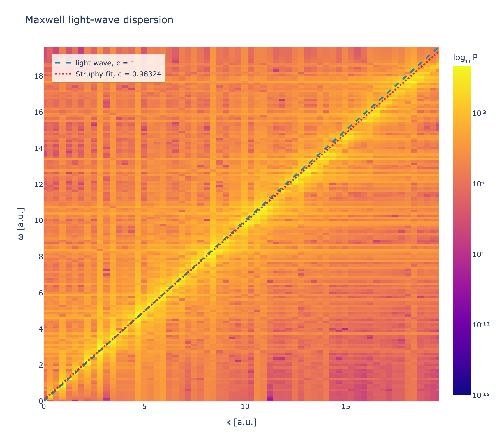
Physical problem
A broadband vacuum light wave
Small deterministic noise perturbations excite several modes of the electric field in a periodic one-dimensional domain. A two-dimensional Fourier spectrum reveals the numerical relation between angular frequency and wavenumber.
PDEs solved by model:
Ampère's law (no current):
Faraday's law:
- Model
- Maxwell
- Domain
- Cuboid (r3=20)
- Grid
- 1 × 1 × 128
- FEEC degree
- 1 × 1 × 3
- Integrator
- Implicit
- Evolution
- 1,000 steps
- Visualization
- Plotly
Complete source
Run the simulation
Requires Struphy 3.2 with compiled kernels and Plotly. Run struphy compile once, then execute python maxwell-wave.py.
"""Verify light-wave dispersion with Struphy's Maxwell model.

This compact gallery example follows Struphy's maintained Maxwell verification
test. It excites a broadband electric field, evolves Maxwell's equations with
FEEC, and plots the numerical dispersion relation against omega = c k.

Requires Struphy 3.2 with compiled kernels (`struphy compile`).
"""

import json
from pathlib import Path

import numpy as np
import plotly.graph_objects as go

from struphy import (
    DerhamOptions,
    EnvironmentOptions,
    Simulation,
    Time,
    domains,
    grids,
    perturbations,
)
from struphy.diagnostics.diagn_tools import power_spectrum_2d
from struphy.models import Maxwell


# Model and structure-preserving Maxwell propagator.
model = Maxwell()
model.propagators.maxwell.options = model.propagators.maxwell.Options(
    algo="implicit",
)

# A periodic one-dimensional domain embedded in 3D.
domain = domains.Cuboid(r3=20.0)
grid = grids.TensorProductGrid(num_elements=(1, 1, 128))
derham_opts = DerhamOptions(degree=(1, 1, 3))
time_opts = Time(dt=0.05, Tend=50.0)

# Broadband noise excites several light-wave modes at once.
model.em_fields.e_field.add_perturbation(
    perturbations.Noise(amp=0.1, comp=0, seed=123),
)
model.em_fields.e_field.add_perturbation(
    perturbations.Noise(amp=0.1, comp=1, seed=123),
)

env = EnvironmentOptions(
    out_folders="struphy_gallery_runs",
    sim_folder="maxwell_light_wave",
)
sim = Simulation(
    model=model,
    name="Maxwell light-wave dispersion",
    description=(
        "Excite a broadband electric field and recover the vacuum dispersion "
        "relation ω = ck with Struphy’s FEEC Maxwell solver."
    ),
    env=env,
    time_opts=time_opts,
    domain=domain,
    grid=grid,
    derham_opts=derham_opts,
)

if __name__ == "__main__":
    # Run, evaluate the FEEC fields on a grid, and load the result.
    sim.run()
    sim.pproc(create_vtk=False)
    sim.load_plotting_data()

    # Struphy's diagnostic computes the (k, omega) spectrum and fits its branch.
    electric_field = sim.spline_values.em_fields.e_field_log.data
    omega, kvec, dispersion, coefficients = power_spectrum_2d(
        electric_field,
        "e_field_log",
        grids=sim.grids_log,
        grids_mapped=sim.grids_phy,
        component=0,
        slice_at=[0, 0, None],
        do_plot=False,
        fit_branches=1,
        noise_level=0.5,
        extr_order=10,
        fit_degree=(1,),
    )

    phase_velocity = float(coefficients[0][0])
    print(f"Measured phase velocity: {phase_velocity:.5f} (exact: 1.0)")

    # Build an interactive Plotly view of the normalized power spectrum.
    omega = np.asarray(omega)
    kvec = np.asarray(kvec)
    power = np.asarray(dispersion) ** 2
    power /= power.max()
    log_power = np.log10(np.clip(power, 1e-15, None))
    fit = np.polyval(np.asarray(coefficients[0]), kvec)

    figure = go.Figure(
        go.Heatmap(
            x=kvec,
            y=omega,
            z=log_power,
            zmin=-15,
            zmax=-1,
            colorscale="Plasma",
            colorbar={
                "title": {"text": "log₁₀ P"},
                "tickvals": [-15, -12, -9, -6, -3],
                "ticktext": ["10⁻¹⁵", "10⁻¹²", "10⁻⁹", "10⁻⁶", "10⁻³"],
            },
            hovertemplate="k=%{x:.3f}<br>ω=%{y:.3f}<br>log₁₀ P=%{z:.2f}<extra></extra>",
        ),
    )
    figure.add_scatter(
        x=kvec,
        y=kvec,
        mode="lines",
        name="light wave, c = 1",
        line={"color": "#168aad", "width": 3, "dash": "dash"},
    )
    figure.add_scatter(
        x=kvec,
        y=fit,
        mode="lines",
        name=f"Struphy fit, c = {phase_velocity:.5f}",
        line={"color": "#d62828", "width": 3, "dash": "dot"},
    )
    figure.update_layout(
        title="Maxwell light-wave dispersion",
        xaxis_title="k [a.u.]",
        yaxis_title="ω [a.u.]",
        template="plotly_white",
        autosize=True,
        legend={
            "x": 0.02,
            "y": 0.98,
            "bgcolor": "rgba(255,255,255,0.82)",
            "bordercolor": "rgba(44,62,80,0.25)",
            "borderwidth": 1,
        },
        margin={"l": 75, "r": 45, "t": 80, "b": 70},
    )
    figure.update_xaxes(range=[0, float(kvec[-1])])
    figure.update_yaxes(range=[0, float(kvec[-1])])

    png_path = Path("maxwell-dispersion.png")
    html_path = Path("maxwell-dispersion.html")
    figure.write_image(png_path, width=1100, height=650, scale=2)
    figure.write_html(
        html_path,
        include_plotlyjs="cdn",
        default_width="100%",
        default_height="100%",
        config={"responsive": True, "displaylogo": False},
    )
    print(f"Saved {png_path.resolve()}")
    print(f"Saved {html_path.resolve()}")

    # Fold this run's measured result into the page metadata that
    # generate_examples.py already wrote for this script's static setup.
    metadata_path = Path("maxwell-wave.metadata.json")
    metadata = json.loads(metadata_path.read_text()) if metadata_path.exists() else {}
    metadata["measuredPhaseVelocity"] = phase_velocity
    metadata["exactPhaseVelocity"] = 1.0
    metadata_path.write_text(json.dumps(metadata, indent=2, ensure_ascii=False))
    print(f"Saved {metadata_path.resolve()}")
Adapted from Struphy’s maintained Maxwell verification test. See the post-processing guide for more ways to inspect the result.