Orszag–Tang vortex

Crossed velocity and magnetic vortices cascade into current sheets and magnetic islands — a classic nonlinear, two-dimensional MHD benchmark.

← All examples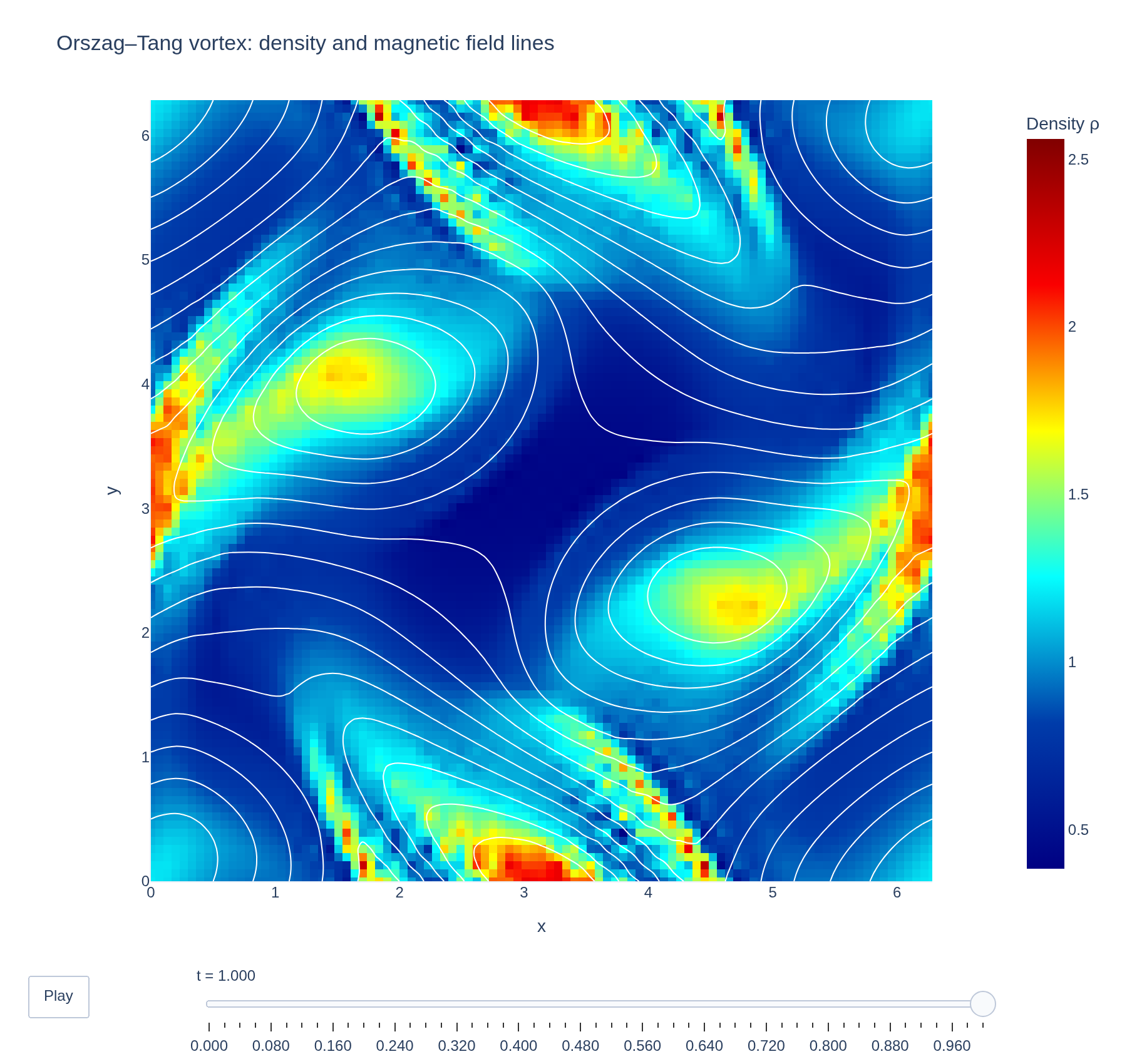

The interactive view is generated from simulated magnetic pressure, animated from the initial crossed vortices to t = 0.005. The static fallback illustrates the characteristic sheets and islands.

Physical problem

A small periodic box that becomes turbulent

The benchmark starts with two simple, divergence-free sine patterns: one for the fluid velocity and one for the magnetic field. Their nonlinear interaction stretches and folds field lines, concentrating current into thin sheets and reconnecting them into magnetic islands. It is a stringent test because the initially smooth solution soon develops sharp structures without losing the magnetic field’s divergence-free constraint.

PDEs solved by model:

Continuity:

\partial_{t} ρ + \nabla \cdot (ρ u) = 0

Momentum:

\partial_{t} (ρ u) + \nabla \cdot (ρ u \otimes u) + ρ \nabla \frac{( ρ U ( ρ , s ))}{\partial ρ} + s \nabla \frac{( ρ U ( ρ , s ))}{\partial s} + B \times \nabla \times B - \nabla \cdot ((μ + μ_{a} (x)) \nabla u) = 0

Entropy:

\partial_{t} s + \nabla \cdot (s u) = \frac{1}{T} ((μ + μ_{a} (x)) ∣\nabla u ∣^{2} + (η + η_{a} (x)) ∣\nabla \times B ∣^{2})

Induction:

\partial_{t} B + \nabla \times (B \times u) + \nabla \times (η + η_{a} (x)) \nabla \times B = 0

where the internal energy per unit mass is :math:`\mathcal U(\rho) = \rho^{\gamma-1} \exp(s / \rho)`, and :math:`\mu_a(\mathbf{x})` and :math:`\eta_a(\mathbf{x})` are artificial viscosity and resistivity coefficients.

Model: ViscoResistiveMHD
Domain: Cuboid (r1=6.28319, r2=6.28319)
Grid: 16 × 16 × 1
FEEC degree: 1 × 1 × 1
Evolution: 1 steps
Visualization: Plotly

Complete source

Run the simulation

Download .py

Requires Struphy 3.3 with compiled kernels and Plotly. Run struphy compile once, then execute python orszag-tang-vortex.py.

"""The Orszag--Tang vortex: a nonlinear 2D MHD turbulence benchmark.

Two crossed, periodic velocity and magnetic-field vortices are evolved with
Struphy's full nonlinear MHD model. Their interaction quickly produces
current sheets and magnetic islands, making this a compact test of nonlinear
field--fluid coupling and the divergence-preserving magnetic discretization.

Requires Struphy 3.3 with compiled kernels (``struphy compile``).
"""

import numpy as np
import plotly.graph_objects as go

from struphy import DerhamOptions, EnvironmentOptions, FieldsBackground, Simulation, Time, domains, equils, grids, perturbations
from struphy.models import ViscoResistiveMHD

# The standard periodic Orszag--Tang initial condition on [0, 2π]².
model = ViscoResistiveMHD(with_viscosity=False, with_resistivity=False)
model.propagators.variat_dens.options = model.propagators.variat_dens.Options(model="full")

domain = domains.Cuboid(r1=2 * np.pi, r2=2 * np.pi, r3=1.0)
# A compact resolution and one stable nonlinear step keep the gallery run
# suitable for CI while exercising the coupled MHD propagators.
grid = grids.TensorProductGrid(num_elements=(16, 16, 1))
derham_opts = DerhamOptions(degree=(1, 1, 1))
time_opts = Time(dt=0.005, Tend=0.005, split_algo="LieTrotter")
# A uniform guide field keeps the otherwise two-dimensional benchmark regular.
equil = equils.HomogenSlab(B0z=1.0, n0=1.0, beta=0.1)

# Uniform density/entropy and zero mean fields, then the two solenoidal
# sine-mode vortices: u = (-sin y, sin x, 0), B = (-sin y, sin 2x, 0).
model.mhd.density.add_background(FieldsBackground(values=(1.0,)))
model.mhd.entropy.add_background(FieldsBackground(values=(0.6,)))
model.mhd.velocity.add_background(FieldsBackground(values=(0.0, 0.0, 0.0)))
model.em_fields.b_field.add_background(FieldsBackground(values=(0.0, 0.0, 0.0)))
model.mhd.velocity.add_perturbation(perturbations.ModesSin(ms=(1,), amps=(-1.0,), Ly=2 * np.pi, comp=0))
model.mhd.velocity.add_perturbation(perturbations.ModesSin(ls=(1,), amps=(1.0,), Lx=2 * np.pi, comp=1))
model.em_fields.b_field.add_perturbation(perturbations.ModesSin(ms=(1,), amps=(-1.0,), Ly=2 * np.pi, comp=0))
model.em_fields.b_field.add_perturbation(perturbations.ModesSin(ls=(2,), amps=(1.0,), Lx=2 * np.pi, comp=1))

env = EnvironmentOptions(out_folders="struphy_gallery_runs", sim_folder="orszag_tang_vortex")
sim = Simulation(
    model=model,
    name="Orszag–Tang vortex",
    description="Crossed velocity and magnetic vortices cascade into current sheets and magnetic islands — a classic nonlinear, two-dimensional MHD benchmark.",
    env=env,
    time_opts=time_opts,
    domain=domain,
    equil=equil,
    grid=grid,
    derham_opts=derham_opts,
)


if __name__ == "__main__":
    from _gallery import merge_metadata, save_figure

    sim.run()
    output = sim.output.process(create_vtk=False)

    b_field = output.fields.em_fields.b_field
    times = np.asarray(b_field.t)
    x, y = b_field.X.isel(e3=0), b_field.Y.isel(e3=0)

    def magnetic_pressure(t):
        field = b_field.sel(t=t).isel(e3=0)
        bx, by = np.asarray(field.isel(component=0)), np.asarray(field.isel(component=1))
        return 0.5 * (bx**2 + by**2)

    frame_indices = np.linspace(0, len(times) - 1, min(80, len(times)), dtype=int)
    frames = [
        go.Frame(name=f"{times[i]:.3f}", data=[go.Heatmap(x=np.asarray(x[:, 0]), y=np.asarray(y[0, :]), z=magnetic_pressure(times[i]).T, colorscale="Turbo")])
        for i in frame_indices
    ]
    figure = go.Figure(data=[go.Heatmap(x=np.asarray(x[:, 0]), y=np.asarray(y[0, :]), z=magnetic_pressure(times[-1]).T, colorscale="Turbo", colorbar={"title": "B² / 2"})], frames=frames)
    figure.update_layout(
        title="Orszag–Tang vortex: magnetic pressure",
        xaxis_title="x",
        yaxis_title="y",
        template="plotly_white",
        margin={"l": 70, "r": 35, "t": 80, "b": 135},
        updatemenus=[{"type": "buttons", "showactive": False, "x": 0, "y": -0.25, "buttons": [{"label": "Play", "method": "animate", "args": [None, {"frame": {"duration": 70, "redraw": True}, "fromcurrent": True}]}]}],
        sliders=[{"active": len(frames) - 1, "x": 0.12, "len": 0.88, "y": -0.17, "currentvalue": {"prefix": "t = "}, "steps": [{"args": [[frame.name], {"frame": {"duration": 0, "redraw": True}, "mode": "immediate"}], "label": frame.name, "method": "animate"} for frame in frames]}],
    )
    figure.update_yaxes(scaleanchor="x", scaleratio=1)
    save_figure(figure, "orszag-tang-vortex", width=900, height=780)
    merge_metadata("orszag-tang-vortex", finalTime=time_opts.Tend)

The Orszag–Tang vortex is a standard nonlinear MHD benchmark. This compact gallery setup uses Struphy’s ViscoResistiveMHD model without its optional dissipative propagators, so it remains compatible with the current API while exercising coupled nonlinear MHD evolution.