Fluid model

ViscoResistiveMHD

Full (non-linear) visco-resistive MHD equations discretized with a variational method.

Overview

ViscoResistiveMHD is the full nonlinear dissipative MHD model in the

entropy formulation. It is the most complete variational MHD model in this family when both viscosity and resistivity are required.

Use cases

This model is appropriate for:

nonlinear dissipative MHD simulations
entropy-based variational MHD benchmarks
studies where both viscosity and resistivity matter

Governing equations

PDEs solved by model:

Continuity:

\partial_{t} ρ + \nabla \cdot (ρ u) = 0

Momentum:

\partial_{t} (ρ u) + \nabla \cdot (ρ u \otimes u) + ρ \nabla \frac{( ρ U ( ρ , s ))}{\partial ρ} + s \nabla \frac{( ρ U ( ρ , s ))}{\partial s} + B \times \nabla \times B - \nabla \cdot ((μ + μ_{a} (x)) \nabla u) = 0

Entropy:

\partial_{t} s + \nabla \cdot (s u) = \frac{1}{T} ((μ + μ_{a} (x)) ∣\nabla u ∣^{2} + (η + η_{a} (x)) ∣\nabla \times B ∣^{2})

Induction:

\partial_{t} B + \nabla \times (B \times u) + \nabla \times (η + η_{a} (x)) \nabla \times B = 0

where the internal energy per unit mass is $U (ρ) = ρ^{γ - 1} exp (s / ρ)$ , and $μ_{a} (x)$ and $η_{a} (x)$ are artificial viscosity and resistivity coefficients.

Normalization

The model uses Alfvén-speed normalization together with entropy-based

thermodynamic units inherited from the chosen internal-energy functional.

Discretization

Time integration is performed by the following propagators (in sequence):

VariationalDensityEvolve
VariationalMomentumAdvection
VariationalEntropyEvolve
VariationalMagFieldEvolve
VariationalViscosity (if with_viscosity is True)
VariationalResistivity (if with_resistivity is True)

Diagnostics

The following scalars are tracked during simulation:

Kinetic energy: en_U
Thermodynamic energy: en_thermo
Magnetic energy: en_mag
Total energy: en_tot
Total density / entropy: dens_tot, entr_tot
Divergence diagnostic: tot_div_B

Examples

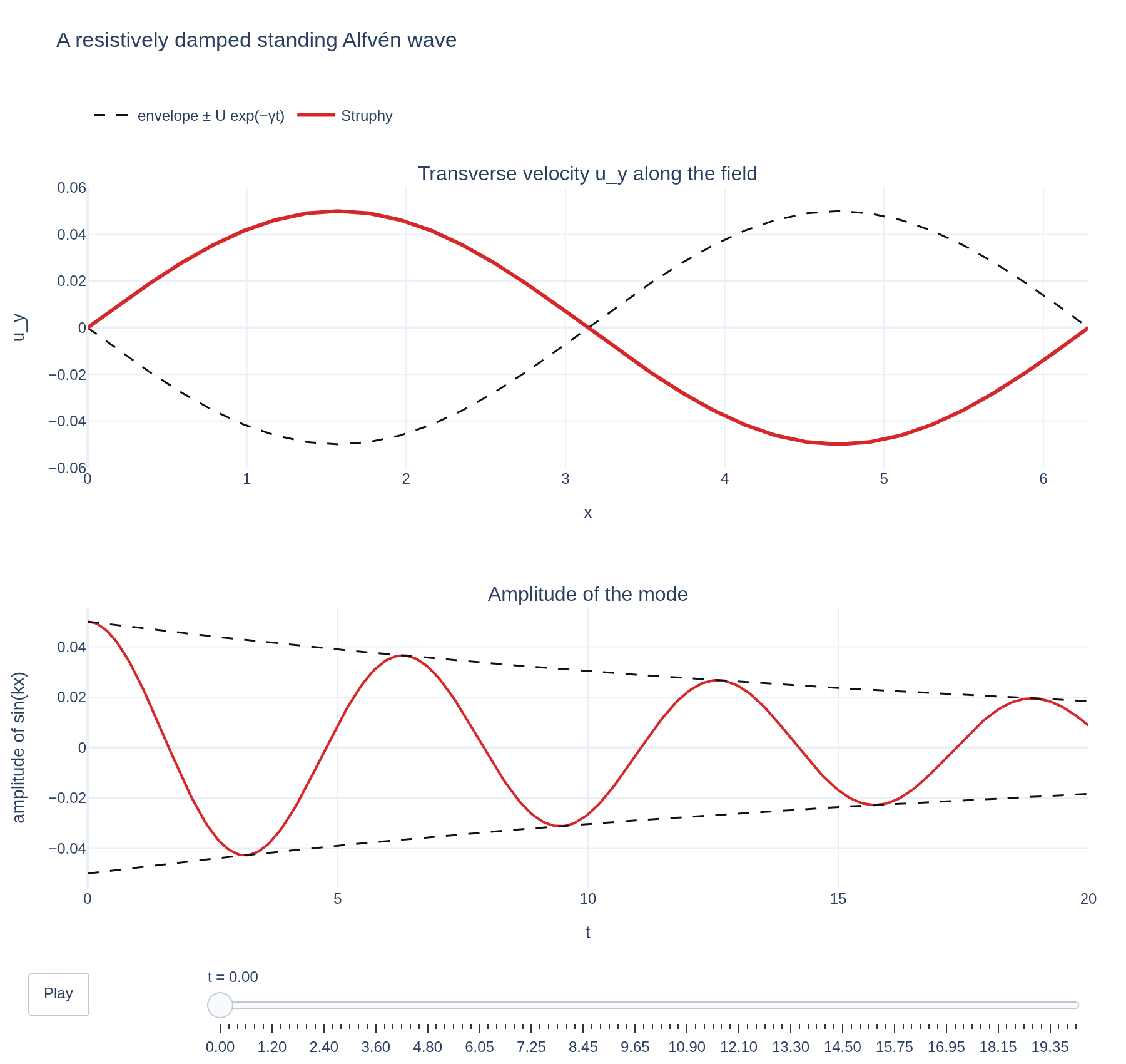
Resistively damped Alfvén wave

A standing Alfvén wave in a resistive plasma oscillates at the Alfvén frequency while its amplitude decays at the rate η k² / 2. Struphy's nonlinear resistive MHD is run at three resistivities and compared with the exact rate. The initial fields are $\mathbf{u}(x,0)=(0,0.05\sin x,0),\qquad \mathbf{B}(x,0)=(1,0,0),$ with $n(x,0)=1$ on $0\le x<2\pi$ ; the scan uses $\eta\in\{0.05,0.1,0.2\}$ .

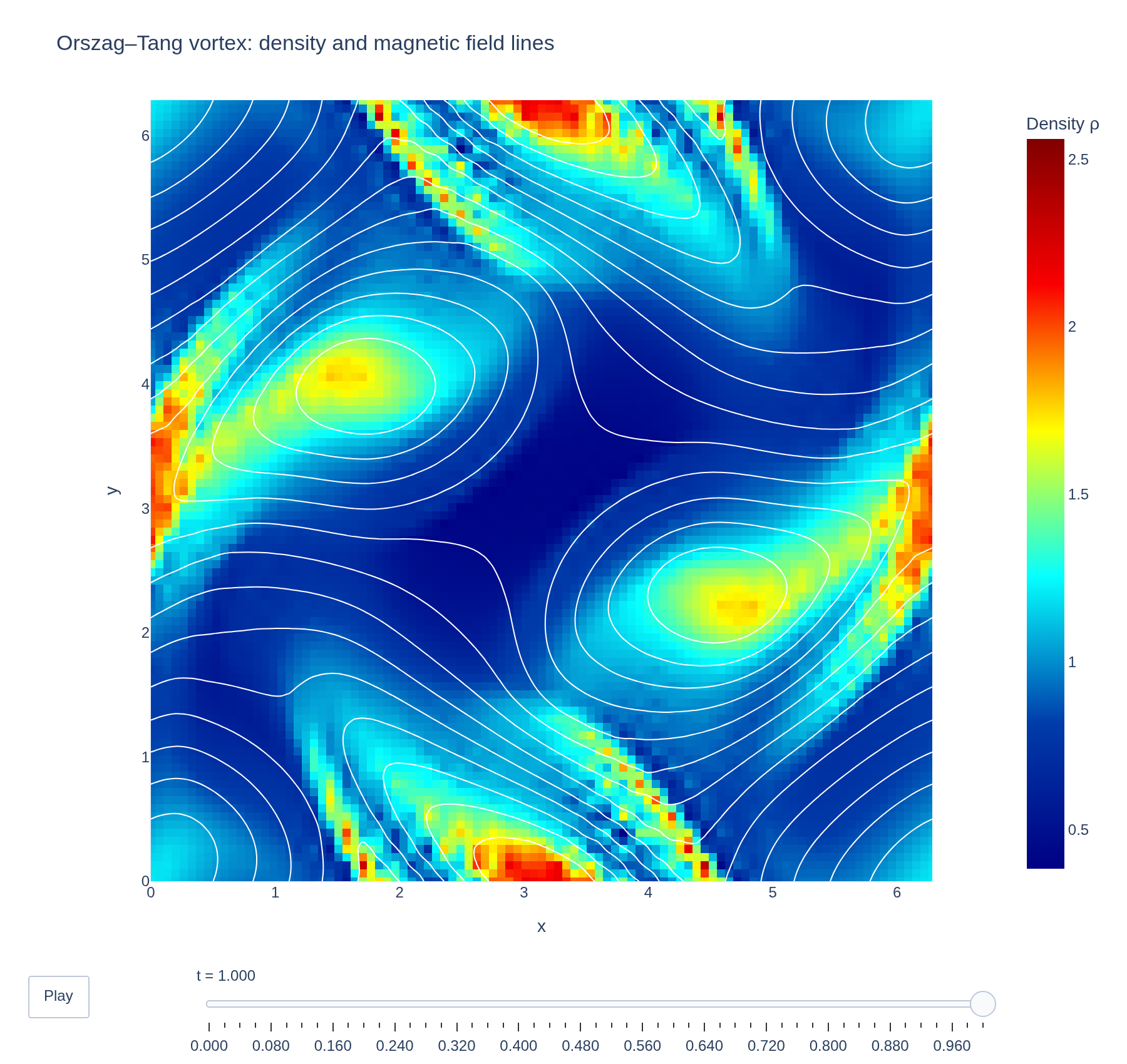
Orszag–Tang vortex

Nonlinear evolution of crossed velocity and magnetic vortices in ideal MHD, with density, magnetic field lines, pressure and conservation diagnostics. The initial vortices are $\mathbf{u}(x,y,0)=(-\sin y,\sin x,0),\qquad \mathbf{B}(x,y,0)=(-\sin y,\sin(2x),0),$ with uniform density $n(x,y,0)=1$ on the periodic square $[0,2\pi)^2$ .

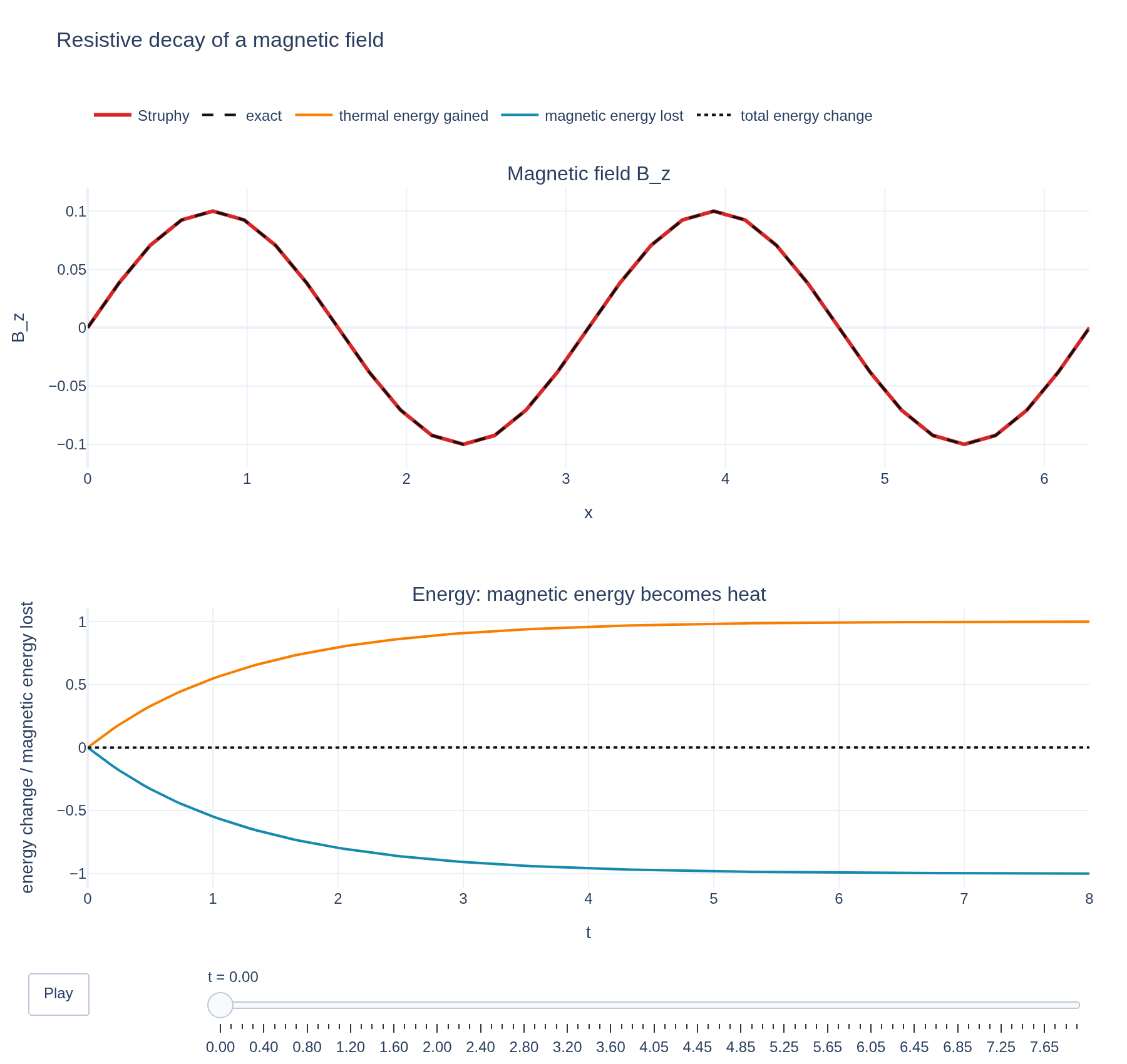
Resistive diffusion of a magnetic field

A sinusoidal magnetic field in a resistive plasma at rest decays without changing shape, at the rate η k². Struphy's variational discretization converts the lost magnetic energy into thermal energy and keeps the total energy constant. The initial state is $\mathbf{B}(x,0)=(0,0,0.1\sin(2x)),\qquad \mathbf{u}(x,0)=0,\qquad n(x,0)=1,$ on $0\le x<2\pi$ , with resistivities $\eta\in\{0.05,0.1,0.2\}$ .

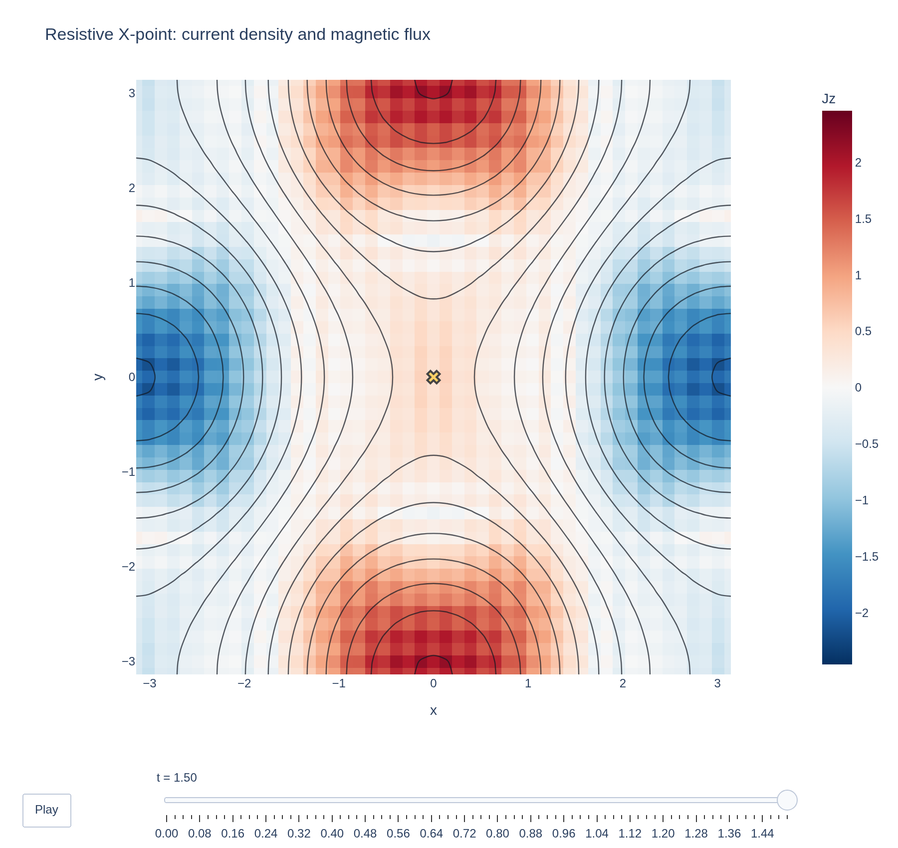
Resistive magnetic X-point

A periodic magnetic X-point is squeezed by an incompressible strain and evolved with Struphy's nonlinear visco-resistive MHD model. Finite resistivity supports an out-of-plane electric field at the null, changes the flux connecting the X- and O-points, and converts magnetic energy into internal energy while the compatible FEEC discretization controls div B. The initial magnetic field and strain are $\mathbf{B}(x,y,0)=(0.7\sin y,\sin x,0),$ $\mathbf{u}(x,y,0)=0.2(-\sin x\cos y,\cos x\sin y,0),$ on $[-\pi,\pi)^2$ , with resistivity $\eta=0.05$ .