Poisson · Electrostatics
Poisson time-dependent source
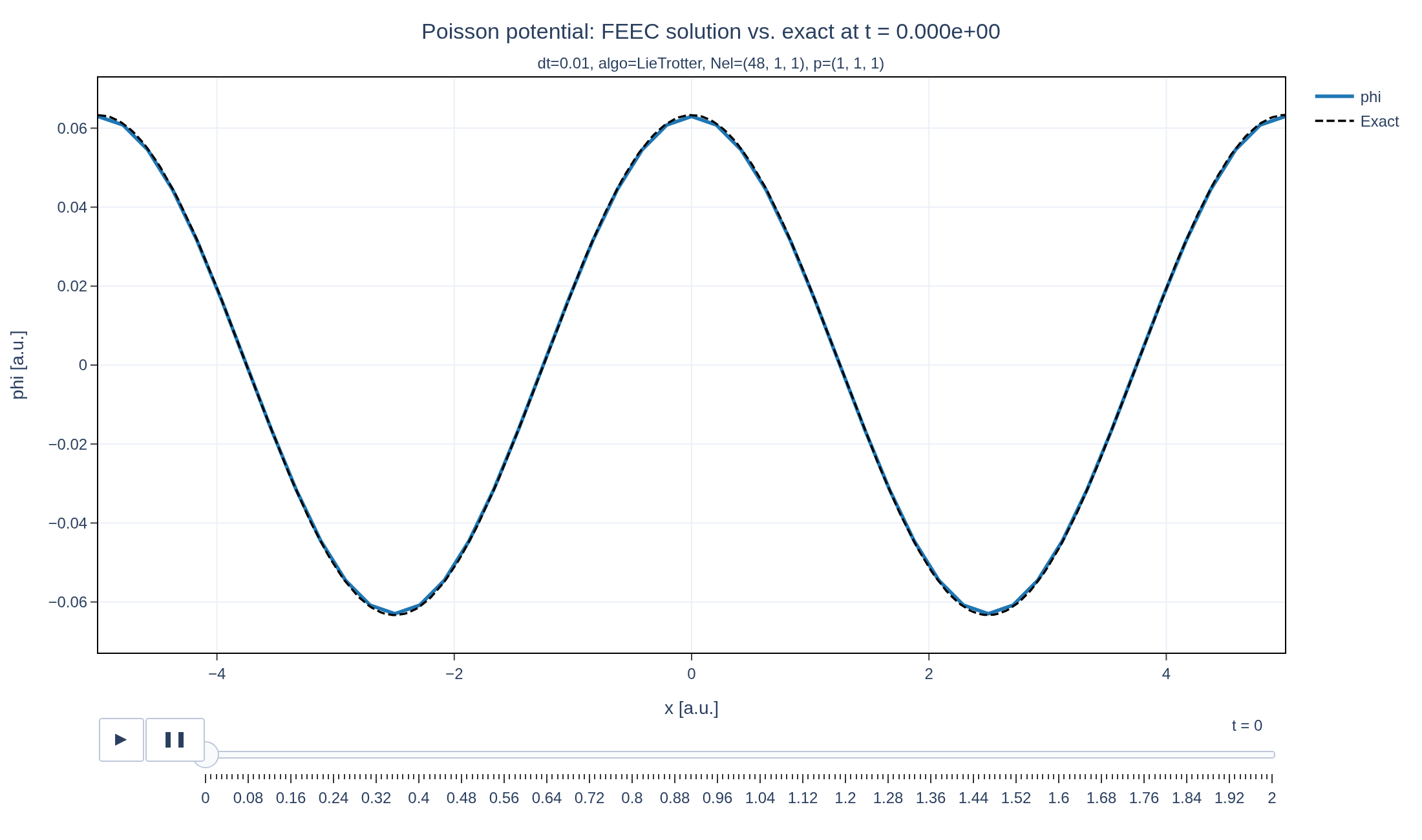
Drive a 1D Poisson solve with an oscillating cosine-mode charge density and compare Struphy’s FEEC potential against the exact solution, at every time step. The prescribed source is on the periodic interval .
Loading interactive figure…
Physical problem
A driven electrostatic potential
PDEs solved by model:
Find such that
where are real-valued functions, is parametrized by time , and is a positive matrix. Boundary terms from integration by parts are assumed to vanish.
Simulation geometry
Domain used in this run
The actual Cuboid geometry reconstructed from this run's metadata. Switch between the 3D view and physical-coordinate slices.
Domain
Cuboid
Mapping
Loading Cuboid…
Parameters
| Parameter | Value | Description |
|---|---|---|
| Loading parameters… | ||
Performance
Profiling
Struphy's built-in scope-profiler instruments every propagator, pusher and solver call — these are the real per-call timings from the run above.
Durations
Gantt (rank 0)
Region statistics
| Region | Count | Avg (s) | Min (s) | Max (s) | Total (s) |
|---|
Complete source
Simulation script
Run it locally
1. Install and compile
Use Python 3.10 or newer with Struphy's system prerequisites installed. Run these commands in your Python environment:
pip install "struphy[pproc]>=3.4.0"
pip install "plasma-plots[plotly]>=0.1.1"
struphy compile
PNG exports need Chrome or Chromium. If Chrome is not installed, run kaleido_get_chrome.
2. Run the script
Download the .py file above, open a terminal in its directory, then run:
python poisson-source.pyFigures are saved in the current directory. Add --show to display them before saving.
"""Verify a time-dependent Poisson solve against its analytic solution.

This compact gallery example follows Struphy's maintained Poisson verification
test. A cosine-mode charge density oscillates in time; Struphy's FEEC solver
recovers the potential at every step, compared here against the closed-form
solution.

Install dependencies and compile the kernels (Python 3.10 or newer):

    pip install "struphy[pproc]>=3.4.0"
    pip install "plasma-plots[plotly]>=0.1.1"
    struphy compile

PNG exports require Chrome or Chromium. If Chrome is not installed, run:

    kaleido_get_chrome

Save this file and run it from the directory where you want the output:

    python poisson-source.py

Figures are saved in the current directory; add --show to display them before saving.
"""

import argparse

import numpy as np
from struphy import (EnvironmentOptions, Simulation, Time, domains, grids,
                     perturbations)
from struphy.models import Poisson
from plasma_plots import save_figure

# Problem parameters: a single cosine mode in space, oscillating in time.
WAVENUMBER = 2
AMPLITUDE = 0.1
OMEGA = 2 * np.pi


def create_simulation() -> Simulation:
    # A time-dependent right-hand side needs the extra `source` propagator.
    model = Poisson(with_t_dep_source=True)

    # A 1D interval, resolved in the x-direction only.
    domain = domains.Cuboid(l1=-5.0, r1=5.0)
    grid = grids.TensorProductGrid(num_elements=(48, 1, 1))
    time_opts = Time(dt=0.01, Tend=2.0)

    # The source oscillates as cos(omega t), driving a single cosine spatial mode.
    model.propagators.source.options = model.propagators.source.Options(omega=OMEGA)

    model.em_fields.source.add_perturbation(
        perturbations.ModesCos(ls=(WAVENUMBER,), amps=(AMPLITUDE,)),
    )

    env = EnvironmentOptions(
        out_folders="struphy_gallery_runs",
        sim_folder="poisson_source",
    )
    simulation = Simulation(
        model=model,
        name="Poisson time-dependent source",
        description=(
            "Drive a 1D Poisson solve with an oscillating cosine-mode charge "
            "density and compare Struphy’s FEEC potential against the exact "
            "solution, at every time step."
            r" The prescribed source is $$\rho(x,t)=0.1\cos(2\pi x/5)\cos(2\pi t),$$"
            r" on the periodic interval :math:`-5\le x<5`."
        ),
        env=env,
        time_opts=time_opts,
        domain=domain,
        grid=grid,
    )
    return simulation


def pproc(sim: Simulation, show: bool = False):
    output = sim.output.pproc(create_vtk=False)
    domain = sim.domain

    # Exact solution of -d^2(phi)/dx^2 = rho(t, x), rho = A cos(k x) cos(omega t).
    Lx = domain.params["r1"] - domain.params["l1"]
    k = WAVENUMBER * 2 * np.pi / Lx

    def phi_exact(x, t):
        return AMPLITUDE / k**2 * np.cos(k * x) * np.cos(OMEGA * t)

    phi = output.fields.em_fields.phi
    phi_line = phi.isel(eta2=0, eta3=0)
    if "component" in phi_line.dims:
        phi_line = phi_line.isel(component=0)
    # The largest pointwise error over the whole run, relative to the amplitude of the exact potential.
    phi_scale = AMPLITUDE / k**2
    max_error = phi_line.plasma.analysis.error(phi_exact, norm="max", dims=("t", "eta1"), args=("X", "t"))
    max_relative_error = float(max_error) / phi_scale
    print(f"Max relative error over the run: {max_relative_error:.5f}")

    figure = phi_line.plasma.plot.line_animation(
        x="eta1",
        reference={"Exact": phi_exact},
        x_of=lambda eta1: domain.params["l1"] + Lx * eta1,
        xlabel="x [a.u.]",
        ylim=(-1.15 * phi_scale, 1.15 * phi_scale),
        title="Poisson potential: FEEC solution vs. exact",
        backend="plotly",
    )

    save_figure(figure, "poisson-source", show=show)


if __name__ == "__main__":
    argparser = argparse.ArgumentParser(description="Run the Poisson source example.")
    argparser.add_argument(
        "--pproc-only",
        action="store_true",
        help="Run post-processing on an existing simulation instead of running a new one.",
    )
    argparser.add_argument("--show", action="store_true", help="Show the figures before saving them.")
    args = argparser.parse_args()

    simulation = create_simulation()

    if args.pproc_only:
        pproc(simulation, show=args.show)
    else:
        simulation.run()
        pproc(simulation, show=args.show)
See the post-processing guide for more ways to inspect the result.