ToyDrift · Electrostatic drift

Vortex merger

Two blobs of charge of the same sign circle each other under E×B drift and merge into one, the guiding-centre analogue of the merger of two like-signed vortices.

← All examples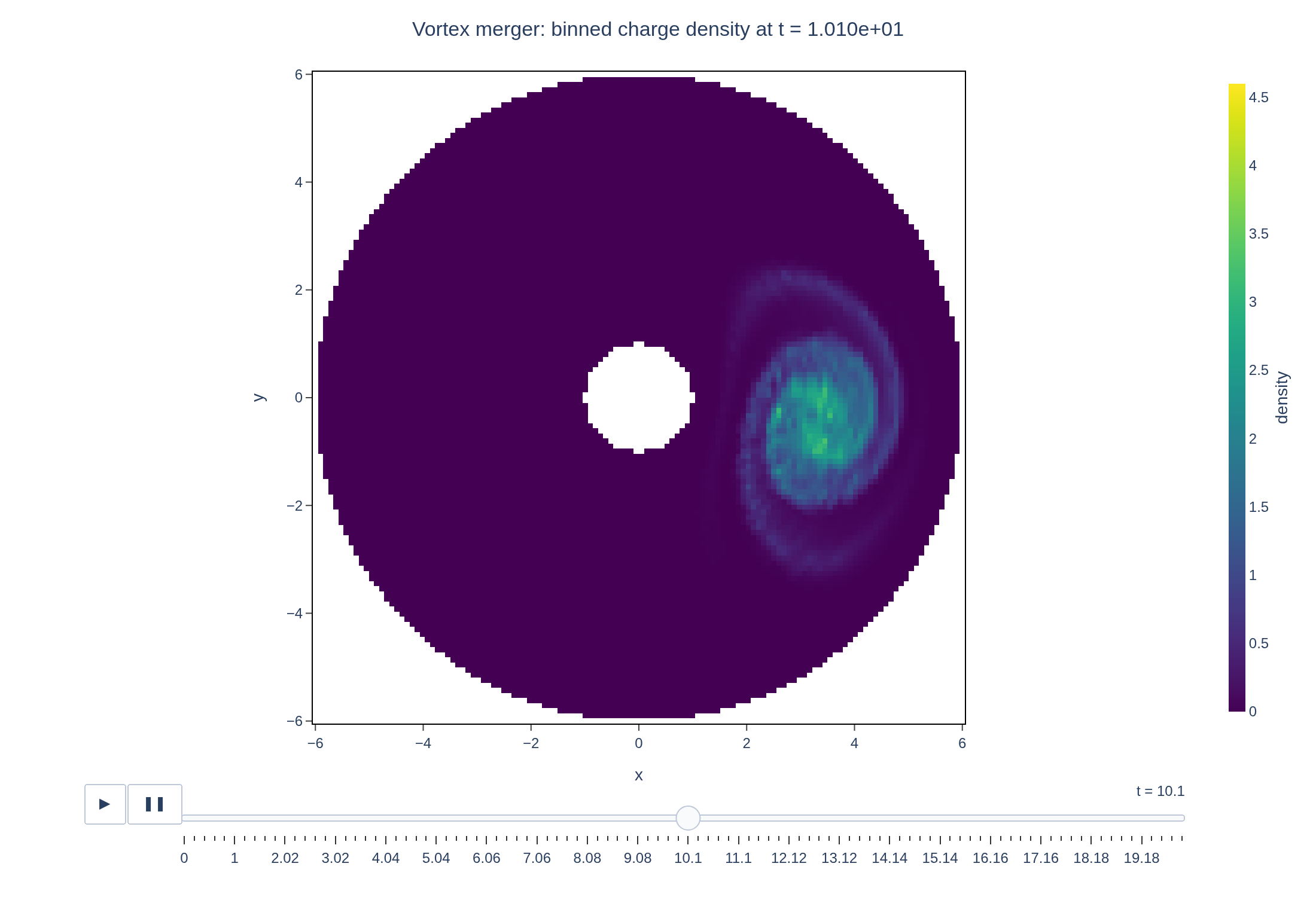

Binned density mapped from radial-angular coordinates to the physical plane. The two initial peaks deform and wind into a common core with surrounding filaments. The animation reaches t = 20; its colour scale is fixed across frames. This finite-resolution calculation retains visible particle noise.

Electrostatic energy relative to the first solved field, at t = 0.02. The t = 0 scalar is an uninitialized zero and is omitted. The drift measures the error of this finite-resolution particle and field calculation; it is not a convergence study.

Physical problem

Two charge blobs in an annulus

Two Gaussian charge blobs are placed on the same circle inside an annulus with grounded radial walls. A uniform magnetic field is perpendicular to the plane. The electrostatic potential follows from Poisson’s equation, and the particles move with the resulting E×B drift. This model has the same advection structure as two-dimensional incompressible vorticity dynamics.

Both blobs have width 0.55, peak density 3 and radial position 3.5; their centres are separated by 2. Their self-consistent flow stretches the density into filaments and forms a shared core. The 48 × 96 diagnostic bins are interpolated onto a Cartesian image with periodic interpolation across the angular seam. The figure shows coarse-grained density, not a claim of irreversible mixing in the continuum equations.

PDEs solved by model:

Drift equation:

\frac{\partial f}{\partial t} + \frac{E \times b _{0}}{B _{∥}^{*}} \cdot \frac{\partial f}{\partial X} = 0

Poisson equation:

- \nabla \cdot \nabla ϕ = \int f B_{∥}^{*} d v_{∥} d μ

where $f (X, v_{∥}, μ, t)$ is the guiding center distribution and

E = - \nabla ϕ, B^{*} = B_{0} + ε v_{∥} \nabla \times b_{0}, B_{∥}^{*} = B^{*} \cdot b_{0}

The control variate method can be activated in the Poisson equation; if enabled, the following Poisson equation is solved:

- \nabla \cdot \nabla ϕ = \int (f - f_{0}) B_{∥}^{*} d v_{∥} d μ

Model: ToyDrift
Domain: HollowCylinder (a2=6, Lz=10)
Grid: 32 × 64 × 1
FEEC degree: 3 × 3 × 1
Integrator: Discrete gradient 1st order newton
Evolution: 1,000 steps
Visualization: Plotly

Performance

Profiling

Download profile .h5

Struphy's built-in scope-profiler instruments every propagator, pusher and solver call — these are the real per-call timings from the run above, rendered live from its data.

Durations

Gantt (rank 0)

Region statistics

Region	Count	Avg (s)	Min (s)	Max (s)	Total (s)

Complete source

Run the simulation

Download .py

Requires the Struphy revision pinned by this site, with compiled kernels, Plotly and Kaleido. Run struphy compile once, then execute python vortex-merger.py.

"""Vortex merger: two like-signed blobs of charge co-rotate and merge.

In a strong magnetic field, a cloud of charge drifts with the E×B velocity of its own electric
field. Two blobs of the same sign therefore circle around each other, and when they start close
enough they merge into one: the guiding-centre analogue of the merger of two like-signed vortices
in a two-dimensional incompressible fluid.

Follows the setup of Struphy's diocotron example (examples/ToyGyrokinetic/diocotron_instability):
an annulus with grounded walls, a uniform background field, and the ToyDrift model.

Requires Struphy 3.2 with compiled kernels (`struphy compile`).
"""

import numpy as np
import plotly.graph_objects as go

from struphy import (
    BaseUnits,
    BinningPlot,
    BoundaryParameters,
    DerhamOptions,
    EnvironmentOptions,
    LoadingParameters,
    SavingParameters,
    Simulation,
    SortingParameters,
    Time,
    WeightsParameters,
    domains,
    equils,
    grids,
    maxwellians,
)
from struphy.models import ToyDrift

model = ToyDrift(epsilon=1.0, alpha=1.0, base_units=BaseUnits(kBT=1.0))

# An annulus between r = 1 and r = 6 with grounded walls and a uniform background field.
domain = domains.HollowCylinder(a1=1.0, a2=6.0, Lz=10.0)
equil = equils.HomogenSlab()
grid = grids.TensorProductGrid(num_elements=(32, 64, 1), mpi_dims_mask=(False, True, False))
derham_opts = DerhamOptions(degree=(3, 3, 1), bcs=(("dirichlet", "dirichlet"), None, None))
time_opts = Time(dt=0.02, Tend=20.0, split_algo="LieTrotter")

# A binned radial-angular density snapshot at every step.
density_bins = BinningPlot(slice="e1_e2", n_bins=(48, 96), ranges=((0.0, 1.0), (0.0, 1.0)))
model.kinetic_ions.set_markers(
    loading_params=LoadingParameters(ppc=60, loading="sobol_standard", spatial="disc"),
    # The markers are loaded over the whole annulus; those outside the blobs carry no weight and are removed.
    weights_params=WeightsParameters(control_variate=True, reject_weights=True, threshold=0.0001),
    boundary_params=BoundaryParameters(),
    sorting_params=SortingParameters(boxes_per_dim=(8, 8, 1), do_sort=True, sorting_frequency=5),
    saving_params=SavingParameters(binning_plots=(density_bins,)),
    bufsize=2.0,
)

model.propagators.gc_poisson.options = model.propagators.gc_poisson.Options()
model.propagators.push_gc_bxe.options = model.propagators.push_gc_bxe.Options(
    algo="discrete_gradient_1st_order_newton",
    evaluate_e_field=True,
)

# Two Gaussian blobs of peak density `peak` and width `width`, on the circle of radius `ring_radius`,
# with their centres `separation` apart.
peak, width, ring_radius, separation = 3.0, 0.55, 3.5, 2.0
half_angle = np.arcsin(separation / (2.0 * ring_radius))
a1, a2 = domain.params["a1"], domain.params["a2"]
centres = [(ring_radius * np.cos(sign * half_angle), ring_radius * np.sin(sign * half_angle)) for sign in (1, -1)]


def two_blobs(etas):
    radius = a1 + (a2 - a1) * etas[:, 0]
    angle = 2.0 * np.pi * etas[:, 1]
    x, y = radius * np.cos(angle), radius * np.sin(angle)
    return sum(peak * np.exp(-((x - cx) ** 2 + (y - cy) ** 2) / (2.0 * width**2)) for cx, cy in centres)


model.kinetic_ions.var.add_background(maxwellians.GyroMaxwellian2D(n=(0.0, None)))
model.kinetic_ions.var.add_initial_condition(maxwellians.GyroMaxwellian2D(n=(two_blobs, None)))

env = EnvironmentOptions(
    out_folders="struphy_gallery_runs",
    sim_folder="vortex_merger",
)
sim = Simulation(
    model=model,
    name="Vortex merger",
    description=(
        "Two blobs of charge of the same sign circle each other under E×B drift "
        "and merge into one, the guiding-centre analogue of the merger of two "
        "like-signed vortices."
    ),
    env=env,
    time_opts=time_opts,
    domain=domain,
    equil=equil,
    grid=grid,
    derham_opts=derham_opts,
)

if __name__ == "__main__":
    import xarray as xr
    from scipy.ndimage import map_coordinates
    from _gallery import export_profiling, heatmap_movie, merge_metadata, publish_thumbnail, save_extra_figure, save_figure

    output = sim.run(profiling_activated=True)
    output.pproc()
    density = output.evaluate("kinetic_ions/e1_e2_density/f")
    times = density.t.values
    if times[-1] < time_opts.Tend - 0.5 * time_opts.dt:
        raise RuntimeError("Vortex-merger simulation ended before the requested final time")

    # Display the radial-angular bins in the physical plane. Pad the angular
    # coordinate periodically so that interpolation is continuous at theta = 0.
    axis = np.linspace(-a2, a2, 128)
    xx, yy = np.meshgrid(axis, axis)
    rr = np.hypot(xx, yy)
    eta_r = (rr - a1) / (a2 - a1)
    eta_theta = np.mod(np.arctan2(yy, xx) / (2 * np.pi), 1.0)
    ir = (eta_r - float(density.e1[0])) / float(density.e1[1] - density.e1[0])
    itheta = (eta_theta - float(density.e2[0])) / float(density.e2[1] - density.e2[0]) + 1
    picks = np.unique(np.linspace(0, len(times) - 1, min(100, len(times)), dtype=int))
    images = []
    for index in picks:
        bins = density.isel(t=index).transpose("e1", "e2").values
        padded = np.pad(bins, ((0, 0), (1, 1)), mode="wrap")
        image = map_coordinates(padded, [ir, itheta], order=1, mode="nearest").astype(np.float32)
        image[(rr < a1) | (rr > a2)] = np.nan
        images.append(image)
    mapped = xr.DataArray(np.array(images), dims=("t", "y", "x"), coords={"t": times[picks], "x": axis, "y": axis})
    figure, _ = heatmap_movie(
        mapped, x="x", y="y", title="Vortex merger: binned charge density",
        xaxis_title="x", yaxis_title="y", colorbar_title="density", zmax=float(density.max()),
    )
    figure.update_xaxes(range=[-a2, a2], constrain="domain")
    figure.update_yaxes(range=[-a2, a2], scaleanchor="x", scaleratio=1)
    still_position = len(figure.frames) // 2
    still = go.Heatmap(figure.data[0])
    still.z = figure.frames[still_position].data[0].z
    save_figure(figure, "vortex-merger", height=750,
                static_data=[still], static_active=still_position)

    # The first Poisson solve initializes the field energy after t=0. Compare
    # subsequent field energies to that first solved state, not to the zero placeholder.
    energy = output.evaluate("en_phi").isel(t=slice(1, None))
    drift = (energy / energy.isel(t=0) - 1).values
    energy_figure = go.Figure(go.Scatter(x=energy.t.values, y=drift, mode="lines", name="field energy"))
    energy_figure.update_layout(title="Vortex merger: electrostatic-energy change", template="plotly_white",
                               xaxis_title="t", yaxis_title="(W − W₁) / W₁", margin={"l": 80, "r": 30, "t": 80, "b": 60})
    figures = [save_extra_figure(
        energy_figure, "vortex-merger", "energy",
        alt="Electrostatic energy change after the first Poisson solve",
        caption="Electrostatic energy relative to the first solved field, at t = 0.02. The t = 0 scalar is an uninitialized zero and is omitted. The drift measures the error of this finite-resolution particle and field calculation; it is not a convergence study.",
    )]
    merge_metadata("vortex-merger", finalTime=float(times[-1]), maxEnergyDrift=float(np.abs(drift).max()),
                   figures=figures, **publish_thumbnail("vortex-merger"), **export_profiling(sim, "vortex-merger"))

Uses the annular ToyDrift setup of the diocotron example, with two Gaussian density peaks in place of the ring.