PressureLessSPH · Pressureless flow
Zel'dovich caustic
A sinusoidal velocity field makes a pressureless gas collapse: the density steepens until it diverges at a caustic, after which the fluid streams through itself. Smoothed particle hydrodynamics follows the collapse and the multi-stream phase space, and is compared with the exact solution of the Lagrangian map.
Run the simulation ↓← All examples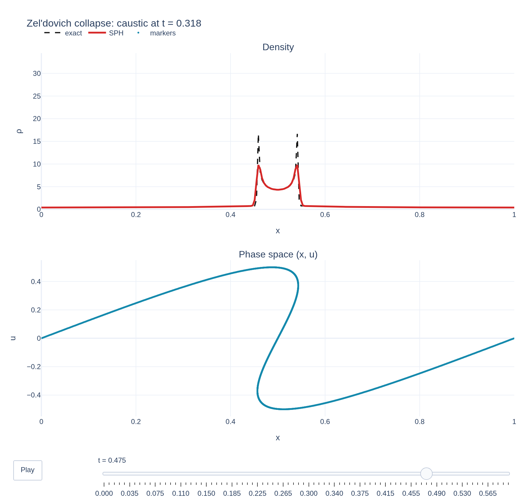
Physical problem
A gas that falls onto itself
A sinusoidal velocity field makes a pressureless gas collapse: the density steepens until it diverges at a caustic, after which the fluid streams through itself. Smoothed particle hydrodynamics follows the collapse and the multi-stream phase space, and is compared with the exact solution of the Lagrangian map.
PDEs solved by model:
Continuity:
Momentum:
where is an external force.
- Model
- PressureLessSPH
- Domain
- Cuboid
- Grid
- 64 × 1 × 1
- FEEC degree
- 3 × 1 × 1
- Evolution
- 120 steps
- Visualization
- Plotly
Performance
Profiling
Struphy's built-in scope-profiler instruments every propagator, pusher and solver call — these are the real per-call timings from the run above.
Gantt (rank 0)
Region statistics
| Region | Count | Avg (s) | Min (s) | Max (s) | Total (s) |
|---|
Complete source
Run the simulation
Requires Struphy with compiled kernels and Plotly. Run struphy compile once, then execute python zeldovich-caustic.py.
"""Caustic formation in pressureless flow: a Zel'dovich collapse with smoothed particle hydrodynamics.

A uniform, pressureless gas is given the velocity u(x) = a sin(2 pi x). Where the velocity converges, the
fluid piles up: the density grows until, at t_c = 1 / (2 pi a), it becomes infinite (a caustic). Afterwards
the fluid streams through itself, and the phase-space curve (x, u) folds over. Every particle keeps its
own velocity, so the exact density at any time follows from the Lagrangian map x = x0 + u(x0) t,

    rho(x, t) = sum over the streams at x of rho_0 / |1 + t u'(x0)|.

The SPH density estimate is compared with it. This is the classic test of pressureless SPH, and the
first stage of the Zel'dovich approximation for structure formation.

Requires Struphy 3.3 with compiled kernels (`struphy compile`).
"""

import numpy as np
import plotly.graph_objects as go

from struphy import (
    BoundaryParameters,
    EnvironmentOptions,
    KernelDensityPlot,
    LoadingParameters,
    SavingParameters,
    Simulation,
    SortingParameters,
    DerhamOptions,
    Time,
    WeightsParameters,
    domains,
    equils,
    grids,
    perturbations,
)
from struphy.models import PressureLessSPH
from struphy.ode.utils import ButcherTableau

amplitude = 0.5  # u(x) = amplitude * sin(2 pi x) on the periodic unit interval
caustic_time = 1.0 / (2 * np.pi * amplitude)  # the density is singular here, at x = 1/2
boxes = 64
markers_per_box = 32
density_points = 256

model = PressureLessSPH()
model.propagators.push_eta.options = model.propagators.push_eta.Options(
    butcher=ButcherTableau(algo="forward_euler"),
)

domain = domains.Cuboid(r1=1.0)
model.cold_fluid.set_markers(
    loading_params=LoadingParameters(ppb=markers_per_box, loading="tesselation"),
    weights_params=WeightsParameters(),
    boundary_params=BoundaryParameters(
        bc=("periodic", "periodic", "periodic"), bc_sph=("periodic", "periodic", "periodic")
    ),
    # The markers pile up at the caustic, so a box must be able to hold many more than its share.
    sorting_params=SortingParameters(
        boxes_per_dim=(boxes, 1, 1), dims_mask=(True, False, False), box_bufsize=30.0
    ),
    saving_params=SavingParameters(
        n_markers=1.0,
        kernel_density_plots=(KernelDensityPlot(pts_e1=density_points, pts_e2=1),),
    ),
)
# Uniform unit density, and the sinusoidal velocity as a perturbation of the (zero) mean flow.
model.cold_fluid.var.add_background(equils.ConstantVelocity(ux=0.0, n=1.0))
model.cold_fluid.var.add_perturbation(del_u1=perturbations.ModesSin(ls=(1,), amps=(amplitude,)))

env = EnvironmentOptions(out_folders="struphy_gallery_runs", sim_folder="zeldovich_caustic")
sim = Simulation(
    model=model,
    name="Zel'dovich caustic",
    description=(
        "A sinusoidal velocity field makes a pressureless gas collapse: the density steepens until it "
        "diverges at a caustic, after which the fluid streams through itself. Smoothed particle "
        "hydrodynamics follows the collapse and the multi-stream phase space, and is compared with the "
        "exact solution of the Lagrangian map."
    ),
    env=env,
    time_opts=Time(dt=0.005, Tend=0.6, split_algo="Strang"),
    domain=domain,
    grid=grids.TensorProductGrid(num_elements=(boxes, 1, 1)),  # for the model's (vanishing) force field
    derham_opts=DerhamOptions(degree=(3, 1, 1)),
)


def exact_density(edges, time, samples=4_000_000):
    """The exact density, averaged over the cells given by `edges`, at `time`.

    Each of `samples` equal fluid elements moves to x = x0 + u(x0) t, so the mass in a cell is the number
    of elements that land in it. This sums over all streams, also after the caustic.
    """
    x0 = (np.arange(samples) + 0.5) / samples
    x = (x0 + amplitude * np.sin(2 * np.pi * x0) * time) % 1.0
    counts, _ = np.histogram(x, bins=edges)
    return counts / samples / np.diff(edges)


if __name__ == "__main__":
    from plotly.subplots import make_subplots

    from _gallery import export_profiling, is_root, merge_metadata, save_figure

    output = sim.run(profiling_activated=True)
    output.pproc()

    density = output.evaluate("cold_fluid/view_0/n").isel(e2=0, e3=0)  # (t, e1): the SPH density estimate
    orbits = output.evaluate("cold_fluid")  # (t, marker, quantity)
    times = orbits.t.values
    assert np.allclose(times, density.t.values)
    grid = density.e1.values
    edges = np.concatenate([[0.0], 0.5 * (grid[1:] + grid[:-1]), [1.0]])
    positions = orbits.sel(quantity="x").values % 1.0  # (t, marker)
    velocities = orbits.sel(quantity="v1").values
    if not (np.isfinite(density.values).all() and np.isfinite(velocities).all()):
        raise RuntimeError("Non-finite SPH result: refusing to publish the run")

    # The relative L1 error of the density estimate, before the caustic (a smooth density) and after it.
    exact = np.array([exact_density(edges, t) for t in times])
    error = np.abs(density.values - exact).sum(axis=1) / exact.sum(axis=1)
    before = times < 0.8 * caustic_time
    after = times > 1.2 * caustic_time
    error_before, error_after = float(error[before].mean()), float(error[after].mean())
    peak_time = float(times[np.argmax(density.values.max(axis=1))])
    if is_root():
        print(f"caustic at t = {caustic_time:.3f}; SPH density peaks at t = {peak_time:.3f}")
        print(f"density error: {100 * error_before:.1f}% before, {100 * error_after:.1f}% after the caustic")

    # Every markers' phase-space position is drawn, so the fold is visible without the exact curve.
    step = max(1, positions.shape[1] // 1500)
    density_ceiling = 1.05 * max(float(exact.max()), float(density.values.max()))

    def traces(index):
        return [
            go.Scatter(x=grid, y=exact[index], mode="lines", name="exact",
                       line={"color": "#111", "width": 2, "dash": "dash"}),
            go.Scatter(x=grid, y=density.values[index], mode="lines", name="SPH",
                       line={"color": "#d62828", "width": 3}),
            go.Scatter(x=positions[index, ::step], y=velocities[index, ::step], mode="markers",
                       marker={"size": 3, "color": "#168aad"}, name="markers", xaxis="x2", yaxis="y2"),
        ]

    picks = np.unique(np.linspace(0, len(times) - 1, min(80, len(times)), dtype=int))
    figure = make_subplots(rows=2, cols=1, vertical_spacing=0.14,
                           subplot_titles=("Density", "Phase space (x, u)"))
    for k, trace in enumerate(traces(0)):
        figure.add_trace(trace, row=1 if k < 2 else 2, col=1)
    figure.frames = [go.Frame(name=f"{times[i]:.3f}", data=traces(i), traces=[0, 1, 2]) for i in picks]
    figure.update_layout(
        title=f"Zel'dovich collapse: caustic at t = {caustic_time:.3f}", template="plotly_white",
        margin={"l": 70, "r": 30, "t": 90, "b": 140}, legend={"orientation": "h", "y": 1.08},
        updatemenus=[{"type": "buttons", "showactive": False, "x": 0, "y": -0.12,
                      "buttons": [{"label": "Play", "method": "animate", "args": [None, {"frame": {"duration": 60, "redraw": True}, "transition": {"duration": 0}, "fromcurrent": True}]}]}],
        sliders=[{"active": 0, "x": 0.12, "len": 0.88, "y": -0.07, "currentvalue": {"prefix": "t = "},
                  "steps": [{"args": [[frame.name], {"frame": {"duration": 0, "redraw": True}, "transition": {"duration": 0}, "mode": "immediate"}], "label": frame.name, "method": "animate"} for frame in figure.frames]}],
    )
    figure.update_xaxes(title_text="x", range=[0, 1], row=1, col=1)
    figure.update_xaxes(title_text="x", range=[0, 1], row=2, col=1)
    figure.update_yaxes(title_text="ρ", range=[0, density_ceiling], row=1, col=1)
    figure.update_yaxes(title_text="u", range=[-1.1 * amplitude, 1.1 * amplitude], row=2, col=1)
    late = int(np.argmin(np.abs(times - 1.5 * caustic_time)))
    save_figure(figure, "zeldovich-caustic", width=900, height=850, static_data=traces(late),
                static_active=int(np.argmin(np.abs(picks - late))))

    merge_metadata(
        "zeldovich-caustic",
        causticTime=caustic_time, sphPeakTime=peak_time, densityErrorBefore=error_before,
        densityErrorAfter=error_after, markers=int(positions.shape[1]),
        **export_profiling(sim, "zeldovich-caustic"),
    )
See the post-processing guide for more ways to inspect the result.