SPH in Beltrami force field#

In this tutorial, you will set up and run a pressure-less SPH example in Struphy, then inspect particle evolution with simple diagnostics.

This notebook focuses on pressure-less flow in a Beltrami force field (model ColdEulerSPH). If you want to start from template parameter files, generate them from the command line:

struphy params ColdEulerSPH

The notebook keeps everything in Python so you can adjust parameters interactively and rerun sections quickly.

Pressure-Less Flow in a Beltrami Force Field#

We begin with a particle system in a 3D box domain \(\Omega \subset \mathbb{R}^3\).

Given an initial velocity field \(\mathbf{u}_0(\mathbf{x})\), we seek trajectories \((\mathbf{x}_p, \mathbf{v}_p)\) for particles \(p=0,\dots,N-1\) satisfying

\[\begin{split}\begin{aligned} \dot{\mathbf x}_p &= \mathbf v_p\,,\qquad && \mathbf x_p(0) = \mathbf x_{p0}\,, \\[2mm] \dot{\mathbf v}_p &= -\nabla p(\mathbf x_p)\,,\qquad && \mathbf v_p(0) = \mathbf u_0(\mathbf x_p(0))\,. \end{aligned}\end{split}\]

Here, \(p \in H^1(\Omega)\) is a prescribed scalar field. In this example, we choose \(p\) so that the force field has Beltrami structure.

In practice, the workflow is: import APIs, define geometry and time stepping, set marker loading, configure propagators, run, and visualize.

First, import the Struphy components used throughout this tutorial.

[1]:

from struphy import (
    BoundaryParameters,
    DerhamOptions,
    EnvironmentOptions,
    LoadingParameters,
    SavingParameters,
    Simulation,
    SortingParameters,
    Time,
    WeightsParameters,
    domains,
    equils,
    grids,
)

Step 1: Create Environment, Time Integrator, and Domain#

Set up a Cartesian (cuboid) domain and use Strang splitting for time integration. These choices define the simulation skeleton before any particle data are attached.

[2]:

# environment options
env = EnvironmentOptions()

# time stepping
time_opts = Time(dt=0.02, Tend=4, split_algo="Strang")

# geometry
l1 = -0.5
r1 = 0.5
l2 = -0.5
r2 = 0.5
l3 = 0.0
r3 = 1.0
domain = domains.Cuboid(l1=l1, r1=r1, l2=l2, r2=r2, l3=l3, r3=r3)

Step 2: Define the Beltrami Background#

Next, define velocity, pressure, and density functions for the background equilibrium. We pass these to GenericCartesianFluidEquilibrium, which will later be used to initialize the particle state.

[3]:

# construct Beltrami flow
import numpy as np


def u_fun(x, y, z):
    ux = -np.cos(np.pi * x) * np.sin(np.pi * y)
    uy = np.sin(np.pi * x) * np.cos(np.pi * y)
    uz = 0 * x
    return ux, uy, uz


p_fun = lambda x, y, z: 0.5 * (np.sin(np.pi * x) ** 2 + np.sin(np.pi * y) ** 2)
n_fun = lambda x, y, z: 1.0 + 0 * x

# put the functions in a generic equilibrium container
bel_flow = equils.GenericCartesianFluidEquilibrium(u_xyz=u_fun, p_xyz=p_fun, n_xyz=n_fun)

Step 3: Choose Grid and de Rham Options#

Even for particle-based dynamics, Struphy uses spline-based projections for some fields. Here we define a tensor-product grid and matching de Rham settings.

[4]:

# fluid equilibrium (can be used as part of initial conditions)
equil = None

# grid
grid = grids.TensorProductGrid(num_elements=(64, 64, 1))

# derham options
bcs = (("free", "free"), ("free", "free"), None)
derham_opts = DerhamOptions(degree=(3, 3, 1), bcs=bcs)

Step 4: Instantiate the `ColdEulerSPH` Simulation#

Create a lightweight model instance and combine it with the environment, domain, and discretization settings from the previous steps.

[5]:

# import model
from struphy.models import ColdEulerSPH

# light-weight model instance
model = ColdEulerSPH(epsilon=1.0)

sim = Simulation(
    model,
    env=env,
    time_opts=time_opts,
    domain=domain,
    equil=equil,
    grid=grid,
    derham_opts=derham_opts,
)

/opt/hostedtoolcache/Python/3.10.22/x64/lib/python3.10/site-packages/struphy/models/species.py:239: UserWarning: Override equation parameter self.epsilon =1.0
  warnings.warn(f"Override equation parameter {self.epsilon =}")

Step 5: Configure Marker Loading and Saving#

Now set particle-marker parameters. In this example we:

load Np=1000 particles
keep default weight construction
apply reflective boundaries in \(x,y\) and periodic in \(z\)
save all markers via n_markers=1.0

We also keep sorting simple with one box per direction for this first run.

[6]:

loading_params = LoadingParameters(Np=1000)
weights_params = WeightsParameters()
boundary_params = BoundaryParameters(bc=("reflect", "reflect", "periodic"))
sorting_params = SortingParameters(boxes_per_dim=(1, 1, 1))
saving_params = SavingParameters(n_markers=1.0)

model.fluid.set_markers(
    loading_params=loading_params,
    weights_params=weights_params,
    boundary_params=boundary_params,
    sorting_params=sorting_params,
    saving_params=saving_params,
)

Step 6: Set Propagator Options#

Configure the particle pushers. The key detail is to pass the Beltrami pressure potential to push_v, so the velocity update uses the intended force field.

[7]:

# propagator options
from struphy import ButcherTableau

butcher = ButcherTableau(algo="forward_euler")
model.propagators.push_eta.options = model.propagators.push_eta.Options(butcher=butcher)

phi = bel_flow.p0
model.propagators.push_v.potential = phi

Step 7: Apply Initial Conditions#

Attach the Beltrami equilibrium as the background state for the cold fluid species. No additional perturbation is added in this tutorial run.

[8]:

# background, perturbations and initial conditions
model.fluid.var.add_background(bel_flow)

Step 8: Run and Visualize#

Execute the simulation pipeline in order:

run() to advance particles in time and get the post-processed Output object

Then plot marker trajectories to inspect how the Beltrami-driven flow evolves.

[9]:

out = sim.run()

Time stepping: 100%|██████████| 200/200 [00:01<00:00, 168.80step/s]

[10]:

out.info()


No post-processed data in /home/runner/work/struphy/struphy/doc/_collections/tutorials/sim_1, processing with default options (call out.pproc(...) to choose them)

Post-processing path /home/runner/work/struphy/struphy/doc/_collections/tutorials/sim_1
/opt/hostedtoolcache/Python/3.10.22/x64/lib/python3.10/site-packages/struphy/models/species.py:239: UserWarning: Override equation parameter self.epsilon =1.0
  warnings.warn(f"Override equation parameter {self.epsilon =}")
Skipping fluid.var backgrounds: Cannot restore initial-condition function: lambdas, nested functions, and closures are not supported.

No feec fields found in hdf5 file, skipping post-processing of fields.
Evaluation of 1000 marker orbits for fluid

100%|██████████| 201/201 [00:00<00:00, 235.82it/s]
Output: /home/runner/work/struphy/struphy/doc/_collections/tutorials/sim_1

Key     Description                                        Load with
------  -------------------------------------------------  ---------
en_kin  scalar time series (en kin)                        out.evaluate('scalars', variables='en_kin')
fluid   marker trajectories (x, y, z, v1, v2, v3, weight)  out.evaluate('fluid/orbits')

Hints
-----
- t=-1 (index), t=slice(...) or t=0.5 (time value) selects snapshots; the t dimension is kept.
- Other keyword arguments select named coordinates, e.g. component=0 or marker=[0, 1, 2].
- Fields: pass eta1=, eta2=, eta3= (scalars or 1D arrays) to evaluate on a logical grid;
  omitted directions default to 0.5. The result carries physical coordinates X, Y, Z.
- Particles: out.info('species/variable') lists alternative datasets for dataset=.
- Orbits are an xarray.Dataset with one (t, marker) variable per quantity, e.g. orbits.x;
  each variable's 'description' attribute says what it is.
- Results are xarray objects: use .sel/.isel, .plot(x='X'), or .values for NumPy.

[11]:

print(out.fluid.orbits)

<xarray.Dataset> Size: 11MB
Dimensions:    (t: 201, marker: 1000)
Coordinates:
  * t          (t) float64 2kB 0.0 0.02 0.04 0.06 0.08 ... 3.94 3.96 3.98 4.0
  * marker     (marker) int64 8kB 0 1 2 3 4 5 6 ... 993 994 995 996 997 998 999
    t_seconds  (t) float64 2kB 0.0 0.02 0.04 0.06 0.08 ... 3.94 3.96 3.98 4.0
Data variables:
    x          (t, marker) float64 2MB ...
    y          (t, marker) float64 2MB ...
    z          (t, marker) float64 2MB ...
    v1         (t, marker) float64 2MB ...
    v2         (t, marker) float64 2MB ...
    v3         (t, marker) float64 2MB ...
    weight     (t, marker) float64 2MB ...
Attributes:
    product:   orbits
    label:     marker orbits
    run:       dt=0.02, algo=Strang, Nel=(64, 64, 1), p=(3, 3, 1)
    run_name:  sim_1

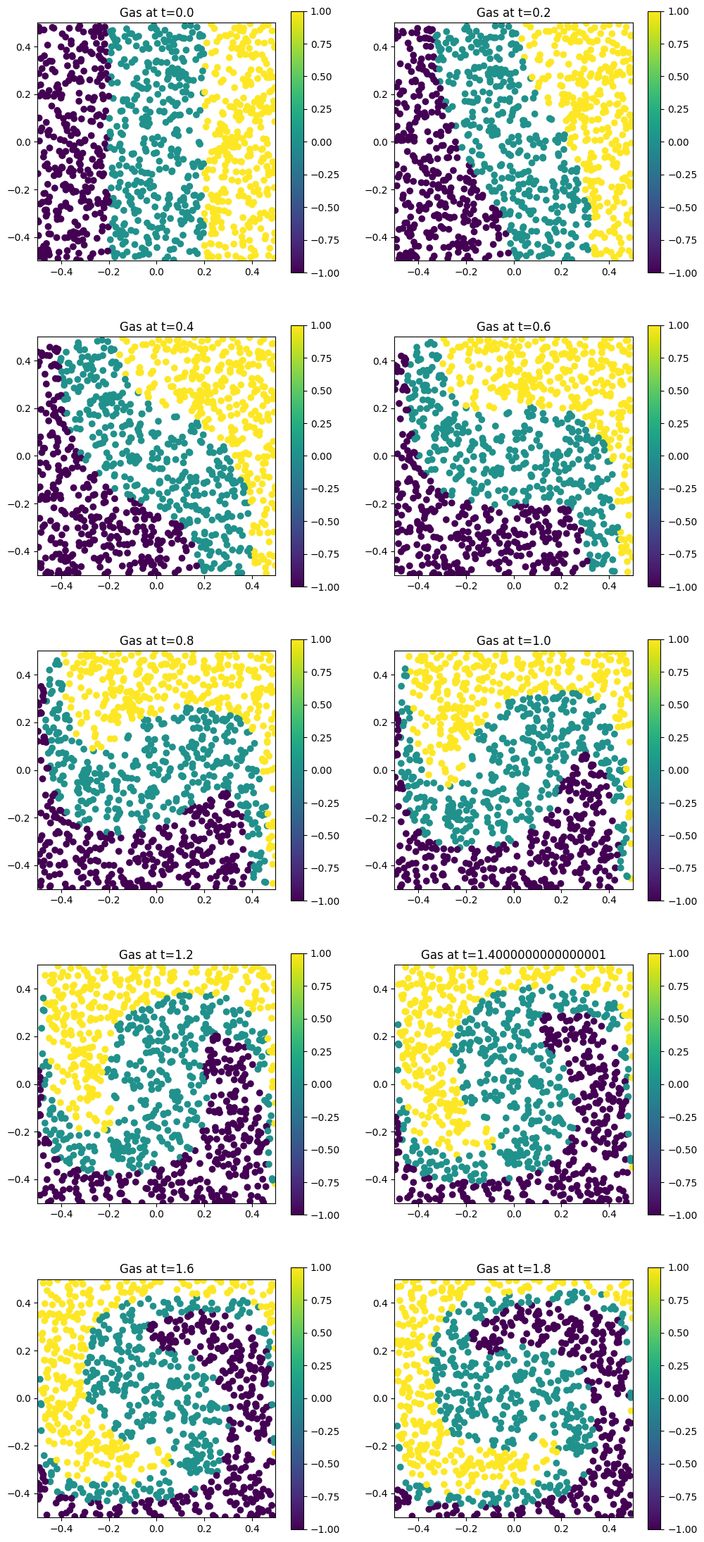
[12]:

from matplotlib import pyplot as plt

plt.figure(figsize=(12, 28))

# one (t, marker) variable per saved quantity: orbits.x, orbits.y, ...
orbits = out.evaluate("fluid/orbits")

coloring = np.select([orbits.x[0] <= -0.2, np.abs(orbits.x[0]) < +0.2, orbits.x[0] >= 0.2], [-1.0, 0.0, +1.0])

dt = time_opts.dt
Nt = out.time.size - 1
interval = Nt / 20
plot_ct = 0
for i in range(Nt):
    if i % interval == 0:
        print(f"{i=}")
        plot_ct += 1
        plt.subplot(5, 2, plot_ct)
        ax = plt.gca()
        plt.scatter(orbits.x[i], orbits.y[i], c=coloring)
        plt.axis("square")
        plt.title("n0_scatter")
        plt.xlim(l1, r1)
        plt.ylim(l2, r2)
        plt.colorbar()
        plt.title(f"Gas at t={i * dt}")
    if plot_ct == 10:
        break

i=0
i=10
i=20
i=30
i=40
i=50
i=60
i=70
i=80
i=90

../../_images/_collections_tutorials_tutorial_beltrami_sph_21_1.png

Step 9: Repeat with Structured Marker Loading#

To compare loading strategies, run a second simulation in a separate folder (sim_2) so outputs stay isolated from the first run.

[13]:

# light-weight model instance
model = ColdEulerSPH(epsilon=1.0)

# environment options
env = EnvironmentOptions(sim_folder="sim_2")

# simulation instance
sim_tess = sim.spawn_sister(model=model, env=env)

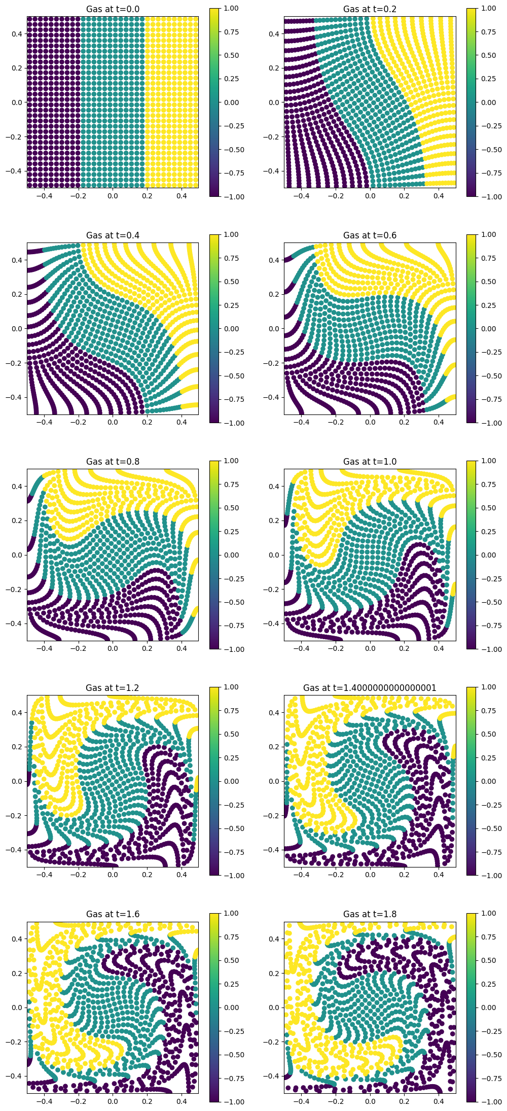
/opt/hostedtoolcache/Python/3.10.22/x64/lib/python3.10/site-packages/struphy/models/species.py:239: UserWarning: Override equation parameter self.epsilon =1.0
  warnings.warn(f"Override equation parameter {self.epsilon =}")

This time, use tessellation-based loading so markers start on a regular grid-like pattern. This gives a useful contrast to random loading when you inspect the trajectory plots.

[14]:

loading_params = LoadingParameters(ppb=4, loading="tesselation")
weights_params = WeightsParameters()
boundary_params = BoundaryParameters(bc=("reflect", "reflect", "periodic"))
sorting_params = SortingParameters(boxes_per_dim=(16, 16, 1))
saving_params = SavingParameters(n_markers=1.0)

model.fluid.set_markers(
    loading_params=loading_params,
    weights_params=weights_params,
    boundary_params=boundary_params,
    sorting_params=sorting_params,
    saving_params=saving_params,
    bufsize=0.5,
)

[15]:

# propagator options
from struphy import ButcherTableau

butcher = ButcherTableau(algo="forward_euler")
model.propagators.push_eta.options = model.propagators.push_eta.Options(butcher=butcher)

phi = bel_flow.p0
model.propagators.push_v.potential = phi

[16]:

# background, perturbations and initial conditions
model.fluid.var.add_background(bel_flow)

[17]:

out_tess = sim_tess.run()

Time stepping: 100%|██████████| 200/200 [00:01<00:00, 147.22step/s]

[18]:

from matplotlib import pyplot as plt

plt.figure(figsize=(12, 28))

# one (t, marker) variable per saved quantity: orbits.x, orbits.y, ...
orbits = out_tess.evaluate("fluid/orbits")

coloring = np.select([orbits.x[0] <= -0.2, np.abs(orbits.x[0]) < +0.2, orbits.x[0] >= 0.2], [-1.0, 0.0, +1.0])

dt = time_opts.dt
Nt = out_tess.time.size - 1
interval = Nt / 20
plot_ct = 0
for i in range(Nt):
    if i % interval == 0:
        print(f"{i=}")
        plot_ct += 1
        plt.subplot(5, 2, plot_ct)
        ax = plt.gca()
        plt.scatter(orbits.x[i], orbits.y[i], c=coloring)
        plt.axis("square")
        plt.title("n0_scatter")
        plt.xlim(l1, r1)
        plt.ylim(l2, r2)
        plt.colorbar()
        plt.title(f"Gas at t={i * dt}")
    if plot_ct == 10:
        break

Skipping fluid.var backgrounds: Cannot restore initial-condition function: lambdas, nested functions, and closures are not supported.

No post-processed data in /home/runner/work/struphy/struphy/doc/_collections/tutorials/sim_2, processing with default options (call out.pproc(...) to choose them)

Post-processing path /home/runner/work/struphy/struphy/doc/_collections/tutorials/sim_2

No feec fields found in hdf5 file, skipping post-processing of fields.
Evaluation of 1024 marker orbits for fluid

100%|██████████| 201/201 [00:00<00:00, 234.56it/s]
i=0
i=10
i=20
i=30
i=40
i=50
i=60
i=70
i=80
i=90

Table of Contents

Previous topic

Next topic

SPH in Beltrami force field#

Pressure-Less Flow in a Beltrami Force Field#

Step 1: Create Environment, Time Integrator, and Domain#

Step 2: Define the Beltrami Background#

Step 3: Choose Grid and de Rham Options#

Step 4: Instantiate the `ColdEulerSPH` Simulation#

Step 5: Configure Marker Loading and Saving#

Step 6: Set Propagator Options#

Step 7: Apply Initial Conditions#

Step 8: Run and Visualize#

Step 9: Repeat with Structured Marker Loading#

Table of Contents

Previous topic

Next topic

SPH in Beltrami force field#

Pressure-Less Flow in a Beltrami Force Field#

Step 1: Create Environment, Time Integrator, and Domain#

Step 2: Define the Beltrami Background#

Step 3: Choose Grid and de Rham Options#

Step 4: Instantiate the ColdEulerSPH Simulation#

Step 5: Configure Marker Loading and Saving#

Step 6: Set Propagator Options#

Step 7: Apply Initial Conditions#

Step 8: Run and Visualize#

Step 9: Repeat with Structured Marker Loading#

Step 4: Instantiate the `ColdEulerSPH` Simulation#