
Profiling Struphy with scope-profiler#
This tutorial shows two ways to use scope-profiler:
Profile a small standalone Python workload with
ProfileManagerregion timing.Configure a Struphy
SimulationwithProfilingOptions, including line profiling, and activate profiling atsim.run(...).
The same HDF5 output file can be inspected from Python, from the command-line interface, or in the terminal TUI.
Imports and output directory#
Use a small temporary directory so repeated notebook runs do not overwrite production simulation data.
[1]:
from pathlib import Path
import shutil
import tempfile

import numpy as np
from scope_profiler import ProfileManager

workdir = Path(tempfile.mkdtemp(prefix="struphy_profile_tutorial_"))
1. Profile standalone Python code#
ProfileManager.profile_region(...) profiles a with block. @ProfileManager.profile(...) profiles a decorated function. This first example only records region timings, which is enough for coarse timing and produces a small HDF5 profile file.
[3]:
@ProfileManager.profile("demo: matrix multiply")
def matrix_work(n: int) -> float:
    a = np.arange(n * n, dtype=float).reshape(n, n)
    b = a.T.copy()
    c = a @ b
    return float(c.sum())


profile_file = workdir / "demo_scope_profile.h5"

with ProfileManager.session(
    file_path=str(profile_file),
    return_results=True,
    verbose=False,
) as prof:
    with ProfileManager.profile_region("demo: total"):
        total = 0.0
        for n in (16, 24, 32):
            total += matrix_work(n)
        print(f"Total sum: {total:.2f}")

results = prof.results
Total sum: 9785934080.00
The context manager finalizes the run and writes one HDF5 file. With return_results=True, the finalized result object is also available in memory.
[4]:
results.print_summary(title="Standalone demo", include=[r"^demo:"])
  ╭──────────────────────────────────────────────╮
  │ region                           total [s]   │
  ├──────────────────────────────────────────────┤
  │ demo: total                      0.000146    │
  │ └─ (own)                            0.000065 │
  │ └─ demo: matrix multiply (3x)       0.000081 │
  ╰──────────────────────────────────────────────╯

  ╭─ Info ─────────────────────────────────────────────────────────────────────────────────────────────────────────────────────────────────────╮
  │ Summary: Standalone demo                                                                                                                   │
  │                                                                                                                                            │
  │ Explore:                                                                                                                                   │
  │   Inspect: scope-profiler inspect ../../../../../../../../tmp/struphy_profile_tutorial_sx58kze1/demo_scope_profile.h5                      │
  │   TUI:     scope-profiler tui ../../../../../../../../tmp/struphy_profile_tutorial_sx58kze1/demo_scope_profile.h5                          │
  │                                                                                                                                            │
  │ Visualize and export:                                                                                                                      │
  │   Plot:    scope-profiler plot default ../../../../../../../../tmp/struphy_profile_tutorial_sx58kze1/demo_scope_profile.h5 -o plots --show │
  │   Report:  scope-profiler report ../../../../../../../../tmp/struphy_profile_tutorial_sx58kze1/demo_scope_profile.h5 -o report.html        │
  │   Export:  scope-profiler export plot-data ../../../../../../../../tmp/struphy_profile_tutorial_sx58kze1/demo_scope_profile.h5 -o data     │
  │   Lines:   scope-profiler line-profile ../../../../../../../../tmp/struphy_profile_tutorial_sx58kze1/demo_scope_profile.h5                 │
  │                                                                                                                                            │
  │ Compare runs:                                                                                                                              │
  │   Diff:    scope-profiler diff BASE.h5 CANDIDATE.h5                                                                                        │
  │   Check:   scope-profiler check BASE.h5 CANDIDATE.h5                                                                                       │
  │                                                                                                                                            │
  │ Durations are in seconds.                                                                                                                  │
  │ Regions may nest, so the summed total can exceed the wall-clock time.                                                                      │
  ╰────────────────────────────────────────────────────────────────────────────────────────────────────────────────────────────────────────────╯
The same file can be inspected from Python. The CLI and TUI commands are shown later for terminal workflows.
[5]:
from scope_profiler import read_h5

standalone_results = read_h5(profile_file)
standalone_results.print_summary(title="Standalone HDF5 summary", include=[r"^demo:"])
  ╭──────────────────────────────────────────────╮
  │ region                           total [s]   │
  ├──────────────────────────────────────────────┤
  │ demo: total                      0.000146    │
  │ └─ (own)                            0.000065 │
  │ └─ demo: matrix multiply (3x)       0.000081 │
  ╰──────────────────────────────────────────────╯

  ╭─ Info ─────────────────────────────────────────────────────────────────────────────────────────────────────────────────────────────────────╮
  │ Summary: Standalone HDF5 summary                                                                                                           │
  │                                                                                                                                            │
  │ Explore:                                                                                                                                   │
  │   Inspect: scope-profiler inspect ../../../../../../../../tmp/struphy_profile_tutorial_sx58kze1/demo_scope_profile.h5                      │
  │   TUI:     scope-profiler tui ../../../../../../../../tmp/struphy_profile_tutorial_sx58kze1/demo_scope_profile.h5                          │
  │                                                                                                                                            │
  │ Visualize and export:                                                                                                                      │
  │   Plot:    scope-profiler plot default ../../../../../../../../tmp/struphy_profile_tutorial_sx58kze1/demo_scope_profile.h5 -o plots --show │
  │   Report:  scope-profiler report ../../../../../../../../tmp/struphy_profile_tutorial_sx58kze1/demo_scope_profile.h5 -o report.html        │
  │   Export:  scope-profiler export plot-data ../../../../../../../../tmp/struphy_profile_tutorial_sx58kze1/demo_scope_profile.h5 -o data     │
  │   Lines:   scope-profiler line-profile ../../../../../../../../tmp/struphy_profile_tutorial_sx58kze1/demo_scope_profile.h5                 │
  │                                                                                                                                            │
  │ Compare runs:                                                                                                                              │
  │   Diff:    scope-profiler diff BASE.h5 CANDIDATE.h5                                                                                        │
  │   Check:   scope-profiler check BASE.h5 CANDIDATE.h5                                                                                       │
  │                                                                                                                                            │
  │ Durations are in seconds.                                                                                                                  │
  │ Regions may nest, so the summed total can exceed the wall-clock time.                                                                      │
  ╰────────────────────────────────────────────────────────────────────────────────────────────────────────────────────────────────────────────╯
2. Profile a Struphy simulation#
Struphy instruments the important phases of Simulation.run() with ProfileManager: allocation and setup, the time-stepping loop (model.integrate), propagators and solvers, diagnostics, particle sorting, and output. A profiling session is only active when sim.run(profiling_activated=True) is called. This means the same Simulation setup can be used for an ordinary run or a measured run.
For a useful performance experiment, keep the problem small enough to run quickly but make the time-stepping loop execute several times. Include a warm-up run when comparing configurations: compilation, cache creation, allocation, and filesystem setup can otherwise dominate the measurement. Use save_step to avoid measuring a workload dominated by output. Start with region timing; enable use_line_profiler=True only after the expensive region is known, because line profiling adds
substantial overhead.
[6]:
from struphy import EnvironmentOptions, ProfilingOptions, Simulation, Time, grids
from struphy.models import Poisson

env = EnvironmentOptions(
    out_folders=str(workdir),
    sim_folder="poisson_profile_demo",
    # Saving every step is useful for a demo, but can dominate a benchmark.
    save_step=1,
)

profiling_opts = ProfilingOptions(
    file_path=str(workdir / "poisson_profile.h5"),
    # First locate the expensive region with region timing.
    use_line_profiler=False,
)

sim = Simulation(
    model=Poisson(),
    env=env,
    time_opts=Time(dt=0.01, Tend=0.01),
    grid=grids.TensorProductGrid(num_elements=(4, 4, 1)),
    profiling_opts=profiling_opts,
)
[7]:
# This profiles the complete Simulation.run() call, including setup,
# model.integrate(), diagnostics, and data output.
sim.run(profiling_activated=True)
struphy_profile_file = Path(profiling_opts.file_path)
WARNING: Class "BasisProjectionOperators" called with degree=(1, 1, 1) (interpolation of piece-wise constants should be avoided).
Stabilizing Poisson solve with self.options.sigma_1 =1e-14
Time stepping: 100%|██████████| 1/1 [00:00<00:00, 177.50step/s]
  ╭──────────────────────────────────────────────────────────────────────────────╮
  │ region                                  % session          total [s]         │
  ├──────────────────────────────────────────────────────────────────────────────┤
  │ scope_profiler.session                  100.00%            0.106586          │
  │ └─ (own)                                   2.98%              0.003176       │
  │ └─ setup: total                            91.94%             0.097999       │
  │ │ └─ (own)                                   0.32%              0.000346     │
  │ │ └─ setup: allocate                         46.52%             0.049585     │
  │ │ │ └─ (own)                                   0.08%              0.000083   │
  │ │ │ └─ setup: feec                             40.93%             0.043628   │
  │ │ │ │ └─ (own)                                   0.08%              0.000090 │
  │ │ │ │ └─ setup: derham                           40.20%             0.042842 │
  │ │ │ │ └─ setup: mass ops                         0.05%              0.000057 │
  │ │ │ │ └─ setup: basis ops                        0.60%              0.000639 │
  │ │ │ └─ setup: variables                        0.27%              0.000284   │
  │ │ │ │ └─ (own)                                   0.13%              0.000141 │
  │ │ │ │ └─ setup var: em_fields.phi                0.09%              0.000098 │
  │ │ │ │ └─ setup var: em_fields.source             0.04%              0.000045 │
  │ │ │ └─ setup: propagators                      3.93%              0.004191   │
  │ │ │ │ └─ (own)                                   0.03%              0.000036 │
  │ │ │ │ └─ setup prop: PoissonSolve                3.90%              0.004155 │
  │ │ │ └─ setup: helpers                          1.31%              0.001399   │
  │ │ │ │ └─ (own)                                   0.89%              0.000952 │
  │ │ │ │ └─ solve: PoissonSolve                     0.37%              0.000392 │
  │ │ │ │ └─ update_feec_variables                   0.05%              0.000055 │
  │ │ └─ setup: run metadata                     0.44%              0.000466     │
  │ │ └─ setup: data storage                     5.35%              0.005700     │
  │ │ └─ setup: geometry vtk                     34.34%             0.036603     │
  │ │ └─ setup: plasma params                    0.66%              0.000700     │
  │ │ └─ setup: initial diagnostics              0.02%              0.000023     │
  │ │ └─ setup: hdf5 datasets                    4.29%              0.004575     │
  │ └─ model.integrate                         0.62%              0.000657       │
  │ │ └─ (own)                                   0.02%              0.000017     │
  │ │ └─ prop: PoissonSolve                      0.60%              0.000640     │
  │ │ │ └─ (own)                                   0.21%              0.000227   │
  │ │ │ └─ solve: PoissonSolve                     0.33%              0.000349   │
  │ │ │ └─ update_feec_variables                   0.06%              0.000064   │
  │ └─ diagnostics                             0.04%              0.000043       │
  │ └─ save data (2x)                          4.42%              0.004711       │
  ╰──────────────────────────────────────────────────────────────────────────────╯

  ╭─ Info ──────────────────────────────────────────────────────────────────────────────────────────────────────────────────────────────────╮
  │ Summary: ../../../../../../../../tmp/struphy_profile_tutorial_sx58kze1/poisson_profile.h5 (1 rank)                                      │
  │                                                                                                                                         │
  │ Explore:                                                                                                                                │
  │   Inspect: scope-profiler inspect ../../../../../../../../tmp/struphy_profile_tutorial_sx58kze1/poisson_profile.h5                      │
  │   TUI:     scope-profiler tui ../../../../../../../../tmp/struphy_profile_tutorial_sx58kze1/poisson_profile.h5                          │
  │                                                                                                                                         │
  │ Visualize and export:                                                                                                                   │
  │   Plot:    scope-profiler plot default ../../../../../../../../tmp/struphy_profile_tutorial_sx58kze1/poisson_profile.h5 -o plots --show │
  │   Report:  scope-profiler report ../../../../../../../../tmp/struphy_profile_tutorial_sx58kze1/poisson_profile.h5 -o report.html        │
  │   Export:  scope-profiler export plot-data ../../../../../../../../tmp/struphy_profile_tutorial_sx58kze1/poisson_profile.h5 -o data     │
  │   Lines:   scope-profiler line-profile ../../../../../../../../tmp/struphy_profile_tutorial_sx58kze1/poisson_profile.h5                 │
  │                                                                                                                                         │
  │ Compare runs:                                                                                                                           │
  │   Diff:    scope-profiler diff BASE.h5 CANDIDATE.h5                                                                                     │
  │   Check:   scope-profiler check BASE.h5 CANDIDATE.h5                                                                                    │
  │                                                                                                                                         │
  │ Durations are in seconds.                                                                                                               │
  │ Regions may nest, so the summed total can exceed the wall-clock time.                                                                   │
  │ % session uses wall-clock coverage; overlapping recursive calls count once.                                                             │
  ╰─────────────────────────────────────────────────────────────────────────────────────────────────────────────────────────────────────────╯
[8]:
from scope_profiler import read_h5

profile_results = read_h5(struphy_profile_file)
region_names = sorted(region.name for region in profile_results.get_regions())
print(", ".join(region_names))
diagnostics, model.integrate, prop: PoissonSolve, save data, scope_profiler.session, setup prop: PoissonSolve, setup var: em_fields.phi, setup var: em_fields.source, setup: allocate, setup: basis ops, setup: data storage, setup: derham, setup: feec, setup: geometry vtk, setup: hdf5 datasets, setup: helpers, setup: initial diagnostics, setup: mass ops, setup: plasma params, setup: propagators, setup: run metadata, setup: total, setup: variables, solve: PoissonSolve, update_feec_variables
Measure setup and time stepping separately#
The profile contains both one-time setup and repeated work. For a performance experiment, inspect them separately: setup is useful for allocation and initialization studies, while model.integrate and its children describe the cost per time step. For a longer benchmark, increase Tend so several steps are recorded, and set save_step larger when output is not part of the question. Include a warm-up run before comparing configurations because compilation, cache creation, allocation, and
filesystem setup can otherwise dominate the measurement.
[9]:
capture_full_output(
    profile_results.print_summary,
    title="What did Simulation.run() measure?",
    include=[r"^setup:", r"^model\.integrate$", r"^prop: ", r"^solve:", r"^kernel: ", r"^save data$"],
)
  ╭──────────────────────────────────────────────────╮
  │ region                           total [s]       │
  ├──────────────────────────────────────────────────┤
  │ setup: total                     0.097999        │
  │ └─ (own)                            0.000346     │
  │ └─ setup: allocate                  0.049585     │
  │ │ └─ (own)                            0.000083   │
  │ │ └─ setup: feec                      0.043628   │
  │ │ │ └─ (own)                            0.000090 │
  │ │ │ └─ setup: derham                    0.042842 │
  │ │ │ └─ setup: mass ops                  0.000057 │
  │ │ │ └─ setup: basis ops                 0.000639 │
  │ │ └─ setup: variables                 0.000284   │
  │ │ └─ setup: propagators               0.004191   │
  │ │ └─ setup: helpers                   0.001399   │
  │ │ │ └─ (own)                            0.000952 │
  │ │ │ └─ solve: PoissonSolve              0.000392 │
  │ └─ setup: run metadata              0.000466     │
  │ └─ setup: data storage              0.005700     │
  │ └─ setup: geometry vtk              0.036603     │
  │ └─ setup: plasma params             0.000700     │
  │ └─ setup: initial diagnostics       0.000023     │
  │ └─ setup: hdf5 datasets             0.004575     │
  │ model.integrate                  0.000657        │
  │ └─ (own)                            0.000017     │
  │ └─ prop: PoissonSolve               0.000640     │
  │ │ └─ (own)                            0.000227   │
  │ │ └─ solve: PoissonSolve              0.000349   │
  │ save data (2x)                   0.004711        │
  ╰──────────────────────────────────────────────────╯

  ╭─ Info ──────────────────────────────────────────────────────────────────────────────────────────────────────────────────────────────────╮
  │ Summary: What did Simulation.run() measure?                                                                                             │
  │                                                                                                                                         │
  │ Explore:                                                                                                                                │
  │   Inspect: scope-profiler inspect ../../../../../../../../tmp/struphy_profile_tutorial_sx58kze1/poisson_profile.h5                      │
  │   TUI:     scope-profiler tui ../../../../../../../../tmp/struphy_profile_tutorial_sx58kze1/poisson_profile.h5                          │
  │                                                                                                                                         │
  │ Visualize and export:                                                                                                                   │
  │   Plot:    scope-profiler plot default ../../../../../../../../tmp/struphy_profile_tutorial_sx58kze1/poisson_profile.h5 -o plots --show │
  │   Report:  scope-profiler report ../../../../../../../../tmp/struphy_profile_tutorial_sx58kze1/poisson_profile.h5 -o report.html        │
  │   Export:  scope-profiler export plot-data ../../../../../../../../tmp/struphy_profile_tutorial_sx58kze1/poisson_profile.h5 -o data     │
  │   Lines:   scope-profiler line-profile ../../../../../../../../tmp/struphy_profile_tutorial_sx58kze1/poisson_profile.h5                 │
  │                                                                                                                                         │
  │ Compare runs:                                                                                                                           │
  │   Diff:    scope-profiler diff BASE.h5 CANDIDATE.h5                                                                                     │
  │   Check:   scope-profiler check BASE.h5 CANDIDATE.h5                                                                                    │
  │                                                                                                                                         │
  │ Durations are in seconds.                                                                                                               │
  │ Regions may nest, so the summed total can exceed the wall-clock time.                                                                   │
  ╰─────────────────────────────────────────────────────────────────────────────────────────────────────────────────────────────────────────╯
Line-profile output for selected Struphy regions#
To get line-by-line timing, repeat the run with use_line_profiler=True (and preferably a shorter Tend). The HDF5 file then contains line-profile records for decorated functions and profiled regions. The filter below prints a representative solver region:
setup: total, the top-level setup block inSimulation.run.solve: PoissonSolve, the Poisson propagator solve call.
The source column is shown because these regions come from real Struphy source files.
[10]:
line_profile_opts = ProfilingOptions(
    file_path=str(workdir / "poisson_line_profile.h5"),
    use_line_profiler=True,
)
line_sim = Simulation(
    model=Poisson(),
    env=EnvironmentOptions(out_folders=str(workdir), sim_folder="poisson_line_demo", save_step=1),
    time_opts=Time(dt=0.01, Tend=0.01),
    grid=grids.TensorProductGrid(num_elements=(4, 4, 1)),
    profiling_opts=line_profile_opts,
)
line_sim.run(profiling_activated=True)
line_profile_file = Path(line_profile_opts.file_path)
WARNING: Class "BasisProjectionOperators" called with degree=(1, 1, 1) (interpolation of piece-wise constants should be avoided).
Stabilizing Poisson solve with self.options.sigma_1 =1e-14
Time stepping: 100%|██████████| 1/1 [00:00<00:00, 86.51step/s]
  ╭──────────────────────────────────────────────────────────────────────────────╮
  │ region                                  % session          total [s]         │
  ├──────────────────────────────────────────────────────────────────────────────┤
  │ scope_profiler.session                  100.00%            0.220734          │
  │ └─ (own)                                   2.64%              0.005818       │
  │ └─ setup: total                            93.57%             0.206530       │
  │ │ └─ (own)                                   2.84%              0.006267     │
  │ │ └─ setup: allocate                         45.30%             0.100001     │
  │ │ │ └─ (own)                                   0.34%              0.000759   │
  │ │ │ └─ setup: feec                             40.05%             0.088401   │
  │ │ │ │ └─ (own)                                   0.64%              0.001419 │
  │ │ │ │ └─ setup: derham                           38.90%             0.085874 │
  │ │ │ │ └─ setup: mass ops                         0.05%              0.000116 │
  │ │ │ │ └─ setup: basis ops                        0.45%              0.000992 │
  │ │ │ └─ setup: variables                        0.45%              0.001004   │
  │ │ │ │ └─ (own)                                   0.30%              0.000670 │
  │ │ │ │ └─ setup var: em_fields.phi                0.08%              0.000180 │
  │ │ │ │ └─ setup var: em_fields.source             0.07%              0.000153 │
  │ │ │ └─ setup: propagators                      3.11%              0.006868   │
  │ │ │ │ └─ (own)                                   0.11%              0.000236 │
  │ │ │ │ └─ setup prop: PoissonSolve                3.00%              0.006631 │
  │ │ │ └─ setup: helpers                          1.35%              0.002969   │
  │ │ │ │ └─ (own)                                   0.92%              0.002023 │
  │ │ │ │ └─ solve: PoissonSolve                     0.38%              0.000830 │
  │ │ │ │ └─ update_feec_variables                   0.05%              0.000116 │
  │ │ └─ setup: run metadata                     0.70%              0.001535     │
  │ │ └─ setup: data storage                     2.81%              0.006201     │
  │ │ └─ setup: geometry vtk                     38.90%             0.085856     │
  │ │ └─ setup: plasma params                    0.38%              0.000845     │
  │ │ └─ setup: initial diagnostics              0.02%              0.000044     │
  │ │ └─ setup: hdf5 datasets                    2.62%              0.005781     │
  │ └─ model.integrate                         0.77%              0.001692       │
  │ │ └─ (own)                                   0.11%              0.000234     │
  │ │ └─ prop: PoissonSolve                      0.66%              0.001458     │
  │ │ │ └─ (own)                                   0.26%              0.000584   │
  │ │ │ └─ solve: PoissonSolve                     0.34%              0.000742   │
  │ │ │ └─ update_feec_variables                   0.06%              0.000133   │
  │ └─ diagnostics                             0.03%              0.000068       │
  │ └─ save data (2x)                          3.00%              0.006625       │
  ╰──────────────────────────────────────────────────────────────────────────────╯

  ╭─ Info ───────────────────────────────────────────────────────────────────────────────────────────────────────────────────────────────────────╮
  │ Summary: ../../../../../../../../tmp/struphy_profile_tutorial_sx58kze1/poisson_line_profile.h5 (1 rank)                                      │
  │                                                                                                                                              │
  │ Explore:                                                                                                                                     │
  │   Inspect: scope-profiler inspect ../../../../../../../../tmp/struphy_profile_tutorial_sx58kze1/poisson_line_profile.h5                      │
  │   TUI:     scope-profiler tui ../../../../../../../../tmp/struphy_profile_tutorial_sx58kze1/poisson_line_profile.h5                          │
  │                                                                                                                                              │
  │ Visualize and export:                                                                                                                        │
  │   Plot:    scope-profiler plot default ../../../../../../../../tmp/struphy_profile_tutorial_sx58kze1/poisson_line_profile.h5 -o plots --show │
  │   Report:  scope-profiler report ../../../../../../../../tmp/struphy_profile_tutorial_sx58kze1/poisson_line_profile.h5 -o report.html        │
  │   Export:  scope-profiler export plot-data ../../../../../../../../tmp/struphy_profile_tutorial_sx58kze1/poisson_line_profile.h5 -o data     │
  │   Lines:   scope-profiler line-profile ../../../../../../../../tmp/struphy_profile_tutorial_sx58kze1/poisson_line_profile.h5                 │
  │                                                                                                                                              │
  │ Compare runs:                                                                                                                                │
  │   Diff:    scope-profiler diff BASE.h5 CANDIDATE.h5                                                                                          │
  │   Check:   scope-profiler check BASE.h5 CANDIDATE.h5                                                                                         │
  │                                                                                                                                              │
  │ Durations are in seconds.                                                                                                                    │
  │ Regions may nest, so the summed total can exceed the wall-clock time.                                                                        │
  │ % session uses wall-clock coverage; overlapping recursive calls count once.                                                                  │
  ╰──────────────────────────────────────────────────────────────────────────────────────────────────────────────────────────────────────────────╯
[11]:
from scope_profiler.line_profile_cli import print_line_profile

print_line_profile(
    line_profile_file,
    region=r"^prop: PoissonSolve",
    display_html=True,
)
Line profile: /tmp/struphy_profile_tutorial_sx58kze1/poisson_line_profile.h5
Rank 0 | prop: PoissonSolve | __call__ (/opt/hostedtoolcache/Python/3.10.21/x64/lib/python3.10/site-packages/struphy/propagators/implicit_diffusion.py:408)
╭────────┬────────┬─────────────┬───────────────┬──────────┬─────────────────────────────────────────────────────────────────────────────────────────╮
│ line │ hits │ time [s] │ per hit [s] │ % time │ source │
├────────┼────────┼─────────────┼───────────────┼──────────┼─────────────────────────────────────────────────────────────────────────────────────────┤
│ 411 │ 1 │ 6.97e-07 │ 6.97e-07 │ 0.05 │ if self._divide_by_dt: │
│ 412 │ │ │ │ │ sig_1 = self._sigma_1 / dt │
│ 413 │ │ │ │ │ sig_2 = self._sigma_2 / dt │
│ 414 │ │ │ │ │ sig_3 = self._sigma_3 / dt │
│ 415 │ │ │ │ │ else: │
│ 416 │ 1 │ 5.78e-07 │ 5.78e-07 │ 0.04 │ sig_1 = self._sigma_1 │
│ 417 │ 1 │ 3.23e-07 │ 3.23e-07 │ 0.02 │ sig_2 = self._sigma_2 │
│ 418 │ 1 │ 3.25e-07 │ 3.25e-07 │ 0.02 │ sig_3 = self._sigma_3 │
│ 419 │ │ │ │ │ │
│ 420 │ │ │ │ │ # compute rhs │
│ 421 │ 1 │ 4.348e-06 │ 4.348e-06 │ 0.30 │ phin = self.variables.phi.spline.vector │
│ 422 │ 1 │ 2.3939e-05 │ 2.3939e-05 │ 1.66 │ rhs = self._stab_mat.dot(phin, out=self._rhs) │
│ 423 │ 1 │ 2.814e-06 │ 2.814e-06 │ 0.19 │ rhs *= sig_2 │
│ 424 │ │ │ │ │ │
│ 425 │ 1 │ 2.411e-06 │ 2.411e-06 │ 0.17 │ self._rhs2 *= 0.0 │
│ 426 │ 2 │ 4.149e-06 │ 2.0745e-06 │ 0.29 │ for src, coeff in zip(self.sources, self.coeffs): │
│ 427 │ 1 │ 1.643e-06 │ 1.643e-06 │ 0.11 │ if isinstance(src, StencilVector): │
│ 428 │ │ │ │ │ self._rhs2 += sig_3 * coeff * src │
│ 429 │ 1 │ 3.7e-07 │ 3.7e-07 │ 0.03 │ elif isinstance(src, FEECVariable): │
│ 430 │ 1 │ 1.543e-06 │ 1.543e-06 │ 0.11 │ v = src.spline.vector │
│ 431 │ 1 │ 0.000184178 │ 0.000184178 │ 12.75 │ self._rhs2 += sig_3 * coeff * self.mass_ops.M0.dot(v, out=self._tmp_src) │
│ 432 │ │ │ │ │ elif isinstance(src, AccumulatorVector): │
│ 433 │ │ │ │ │ if src.particles.control_variate: │
│ 434 │ │ │ │ │ src.particles.update_weights() │
│ 435 │ │ │ │ │ │
│ 436 │ │ │ │ │ if src.space_id == "H1": │
│ 437 │ │ │ │ │ src() # accumulate │
│ 438 │ │ │ │ │ vec = src.vectors[0] │
│ 439 │ │ │ │ │ elif src.space_id == "Hcurl": │
│ 440 │ │ │ │ │ # 1. update density at marker positions │
│ 441 │ │ │ │ │ eta = src.particles.positions │
│ 442 │ │ │ │ │ valid_mks = src.particles.valid_mks │
│ 443 │ │ │ │ │ first_free_idx = src.particles.first_free_idx │
│ 444 │ │ │ │ │ density = src.particles.f0.n0(eta) │
│ 445 │ │ │ │ │ │
│ 446 │ │ │ │ │ src.particles.markers[valid_mks, first_free_idx] = density │
│ 447 │ │ │ │ │ # 2. accumulate │
│ 448 │ │ │ │ │ src() │
│ 449 │ │ │ │ │ # 3. take weak divergence │
│ 450 │ │ │ │ │ vec = -self.derham.grad.T.dot(src.vectors[0], out=self._tmp_src) │
│ 451 │ │ │ │ │ else: │
│ 452 │ │ │ │ │ raise ValueError(f"Unsupported source space {src.space_id}.") │
│ 453 │ │ │ │ │ │
│ 454 │ │ │ │ │ self._rhs2 += sig_3 * coeff * vec │
│ 455 │ │ │ │ │ │
│ 456 │ 1 │ 2.697e-06 │ 2.697e-06 │ 0.19 │ rhs += self._rhs2 │
│ 457 │ │ │ │ │ │
│ 458 │ 1 │ 4.02e-07 │ 4.02e-07 │ 0.03 │ if self.diagnostic is not None: │
│ 459 │ │ │ │ │ proj = L2Projector("H1", self.mass_ops) │
│ 460 │ │ │ │ │ self.diagnostic.spline.vector = proj.solve(rhs) │
│ 461 │ │ │ │ │ │
│ 462 │ │ │ │ │ # compute lhs │
│ 463 │ 1 │ 0.000102956 │ 0.000102956 │ 7.13 │ self._solver.linop = sig_1 * self._stab_mat + self._diffusion_op │
│ 464 │ │ │ │ │ │
│ 465 │ │ │ │ │ # solve │
│ 466 │ 2 │ 0.00023184 │ 0.00011592 │ 16.05 │ with ProfileManager.profile_region(self._solve_region, functions=[self._solver.solve]): │
│ 467 │ 1 │ 0.000732357 │ 0.000732357 │ 50.69 │ out = self._solver.solve(rhs, out=self._tmp) │
│ 468 │ 1 │ 4.84e-07 │ 4.84e-07 │ 0.03 │ info = self._solver._info │
│ 469 │ │ │ │ │ │
│ 470 │ 1 │ 5.38e-07 │ 5.38e-07 │ 0.04 │ if self._info: │
│ 471 │ │ │ │ │ logger.warning(f"\nSolver info: {info}") │
│ 472 │ │ │ │ │ │
│ 473 │ 1 │ 0.000146258 │ 0.000146258 │ 10.12 │ self.update_feec_variables(phi=out) │
╰────────┴────────┴─────────────┴───────────────┴──────────┴─────────────────────────────────────────────────────────────────────────────────────────╯
For a parameter file generated by struphy params <ModelName>, the same pattern is:
profiling_opts = ProfilingOptions(
    file_path="my_profile.h5",
    use_line_profiler=True,
)

sim = Simulation(..., profiling_opts=profiling_opts)
sim.run(profiling_activated=True)
Omit the profiling_activated keyword for normal production runs without profiling overhead.
3. Plot and inspect the profile#
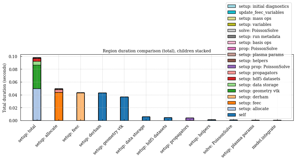
There are three useful levels of inspection: the summary table finds expensive regions; the duration chart ranks them; and the Gantt/flame views explain when they run and how parent/child time is composed. A region’s inclusive duration includes its children, so do not add the model.integrate, propagator, solver, and kernel bars together unless you intentionally want overlapping costs.
scope-profiler also provides a CLI and a terminal TUI for interactive work outside the notebook:
scope-profiler inspect profiling_data.h5
scope-profiler line-profile profiling_data.h5
scope-profiler plot durations profiling_data.h5 -o figures --sort-by total --top-n 20
scope-profiler plot durations profiling_data.h5 -o figures --stack-children --sort-by total --top-n 12
scope-profiler plot gantt profiling_data.h5 -o figures --min-duration 0.0001 --collapse-depth 4
scope-profiler plot flame_graph profiling_data.h5 -o figures
scope-profiler plot flame_chart profiling_data.h5 -o figures
scope-profiler plot quick profiling_data.h5 -o figures
scope-profiler tui profiling_data.h5
We recommend checking out the scope-profiler documentation for details on postprocessing using the tool.
The --stack-children option splits each duration bar into self time plus direct children. Use --collapse-depth and --min-duration to make a busy Gantt chart readable. flame_graph aggregates call stacks; flame_chart preserves their time position.
IPython magics#
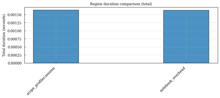
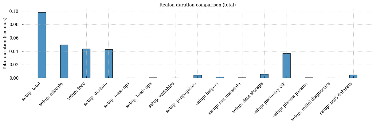
The magics are useful for quick notebook experiments and comparisons. %%scope records a notebook cell as one named region; %scope_load imports the HDF5 profile produced by sim.run() into the same in-memory registry. Use the Struphy HDF5 profile for detailed nested run data, and magics for small local measurements or before/after comparisons.
[12]:
%load_ext scope_profiler.ipython_magics
[13]:
%%scope notebook_overhead -p
sum(i * i for i in range(10_000))
[13]:
333283335000
%%scope 'notebook_overhead'
  ╭──────────────────────────────────────────────────────╮
  │ region                    % session      total [s]   │
  ├──────────────────────────────────────────────────────┤
  │ scope_profiler.session    100.00%        0.001647    │
  │ └─ (own)                     0.80%          0.000013 │
  │ └─ notebook_overhead         99.20%         0.001633 │
  ╰──────────────────────────────────────────────────────╯
[14]:
%scope_load {struphy_profile_file} -n struphy_run -q
%scope_last struphy_run --include ^setup: -p
'struphy_run' (last)
  ╭──────────────────────────────────────────────────╮
  │ region                           total [s]       │
  ├──────────────────────────────────────────────────┤
  │ setup: total                     0.097999        │
  │ └─ (own)                            0.000346     │
  │ └─ setup: allocate                  0.049585     │
  │ │ └─ (own)                            0.000083   │
  │ │ └─ setup: feec                      0.043628   │
  │ │ │ └─ (own)                            0.000090 │
  │ │ │ └─ setup: derham                    0.042842 │
  │ │ │ └─ setup: mass ops                  0.000057 │
  │ │ │ └─ setup: basis ops                 0.000639 │
  │ │ └─ setup: variables                 0.000284   │
  │ │ └─ setup: propagators               0.004191   │
  │ │ └─ setup: helpers                   0.001399   │
  │ └─ setup: run metadata              0.000466     │
  │ └─ setup: data storage              0.005700     │
  │ └─ setup: geometry vtk              0.036603     │
  │ └─ setup: plasma params             0.000700     │
  │ └─ setup: initial diagnostics       0.000023     │
  │ └─ setup: hdf5 datasets             0.004575     │
  ╰──────────────────────────────────────────────────╯
Other useful magics are %%scope_line for a short decorated function, %%scope_recursive for exploratory tracing when no regions exist, %scope_df for pandas analysis, %scope_compare for two notebook runs, and %scope_export for .prof or speedscope output. Recursive tracing is noisy and expensive, so use it to discover candidate functions rather than to measure production performance.
[15]:
capture_full_output(
    profile_results.print_summary,
    title="Poisson profiling summary",
    include=[r"^setup:", r"^model\.integrate$", r"^prop: ", r"^solve:", r"^update_feec_variables$"],
)
  ╭──────────────────────────────────────────────────╮
  │ region                           total [s]       │
  ├──────────────────────────────────────────────────┤
  │ setup: total                     0.097999        │
  │ └─ (own)                            0.000346     │
  │ └─ setup: allocate                  0.049585     │
  │ │ └─ (own)                            0.000083   │
  │ │ └─ setup: feec                      0.043628   │
  │ │ │ └─ (own)                            0.000090 │
  │ │ │ └─ setup: derham                    0.042842 │
  │ │ │ └─ setup: mass ops                  0.000057 │
  │ │ │ └─ setup: basis ops                 0.000639 │
  │ │ └─ setup: variables                 0.000284   │
  │ │ └─ setup: propagators               0.004191   │
  │ │ └─ setup: helpers                   0.001399   │
  │ │ │ └─ (own)                            0.000952 │
  │ │ │ └─ solve: PoissonSolve              0.000392 │
  │ │ │ └─ update_feec_variables            0.000055 │
  │ └─ setup: run metadata              0.000466     │
  │ └─ setup: data storage              0.005700     │
  │ └─ setup: geometry vtk              0.036603     │
  │ └─ setup: plasma params             0.000700     │
  │ └─ setup: initial diagnostics       0.000023     │
  │ └─ setup: hdf5 datasets             0.004575     │
  │ model.integrate                  0.000657        │
  │ └─ (own)                            0.000017     │
  │ └─ prop: PoissonSolve               0.000640     │
  │ │ └─ (own)                            0.000227   │
  │ │ └─ solve: PoissonSolve              0.000349   │
  │ │ └─ update_feec_variables            0.000064   │
  ╰──────────────────────────────────────────────────╯

  ╭─ Info ──────────────────────────────────────────────────────────────────────────────────────────────────────────────────────────────────╮
  │ Summary: Poisson profiling summary                                                                                                      │
  │                                                                                                                                         │
  │ Explore:                                                                                                                                │
  │   Inspect: scope-profiler inspect ../../../../../../../../tmp/struphy_profile_tutorial_sx58kze1/poisson_profile.h5                      │
  │   TUI:     scope-profiler tui ../../../../../../../../tmp/struphy_profile_tutorial_sx58kze1/poisson_profile.h5                          │
  │                                                                                                                                         │
  │ Visualize and export:                                                                                                                   │
  │   Plot:    scope-profiler plot default ../../../../../../../../tmp/struphy_profile_tutorial_sx58kze1/poisson_profile.h5 -o plots --show │
  │   Report:  scope-profiler report ../../../../../../../../tmp/struphy_profile_tutorial_sx58kze1/poisson_profile.h5 -o report.html        │
  │   Export:  scope-profiler export plot-data ../../../../../../../../tmp/struphy_profile_tutorial_sx58kze1/poisson_profile.h5 -o data     │
  │   Lines:   scope-profiler line-profile ../../../../../../../../tmp/struphy_profile_tutorial_sx58kze1/poisson_profile.h5                 │
  │                                                                                                                                         │
  │ Compare runs:                                                                                                                           │
  │   Diff:    scope-profiler diff BASE.h5 CANDIDATE.h5                                                                                     │
  │   Check:   scope-profiler check BASE.h5 CANDIDATE.h5                                                                                    │
  │                                                                                                                                         │
  │ Durations are in seconds.                                                                                                               │
  │ Regions may nest, so the summed total can exceed the wall-clock time.                                                                   │
  ╰─────────────────────────────────────────────────────────────────────────────────────────────────────────────────────────────────────────╯
[16]:
from scope_profiler import plot_durations, plot_flame, plot_gantt

include_regions = [
    r"^setup:",
    r"^model\.integrate$",
    r"^prop: ",
    r"^solve:",
    r"^kernel: ",
    r"^update_feec_variables$",
]
[17]:
duration_figure, _ = plot_durations(
    profile_results,
    include=include_regions,
    sort_by="total",
    top_n=12,
    stack_children=True,
    filepath=str(workdir / "durations_with_children.png"),
    return_fig=True,
)
Plotting duration comparison (total) for files: poisson_profile
[18]:
gantt_figure, _ = plot_gantt(
    profile_results,
    include=include_regions,
    min_duration=1e-4,
    collapse_depth=4,
    filepath=str(workdir / "gantt.png"),
    return_fig=True,
)

flame_figure = plot_flame(
    profile_results,
    include=include_regions,
    filepath=str(workdir / "flame_graph.png"),
    return_fig=True,
)
Plotting Gantt chart for ranks: [0]
Plotting flame chart for: poisson_profile (rank 0)
For interactive flame-chart hover details, use --backend plotly.
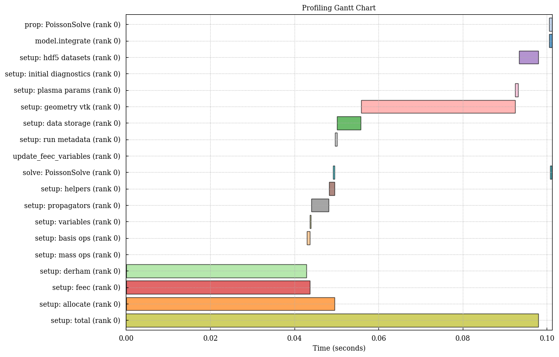
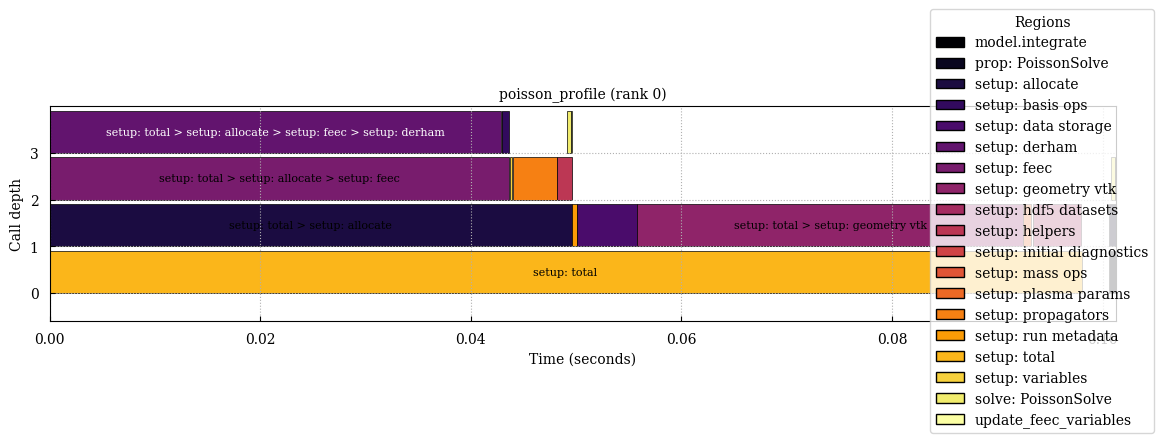
The duration chart ranks regions by aggregate time and stacks self time with direct children. The Gantt chart shows the execution timeline and can expose idle time, serialization, or rank imbalance. The flame graph reconstructs nested calls and is useful for reading parent/child relationships between setup, model.integrate, propagators, solvers, and kernels. The figures are also saved under workdir, so the same workflow works in a headless batch job.
Cleanup#
Remove the temporary directory when you no longer need the profiling files.
[19]:
# shutil.rmtree(workdir)