LinearExtendedMHDuniform · MHD waves
Whistler and ion-cyclotron waves in Hall MHD
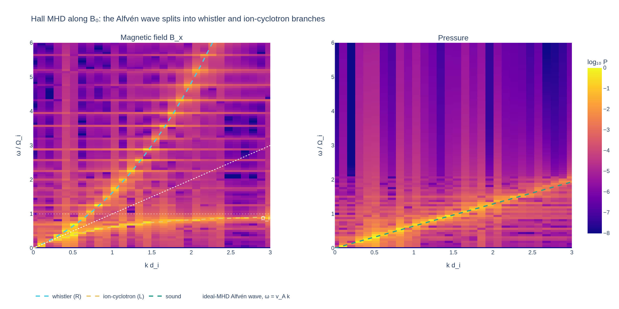
Broadband noise in a uniform magnetized plasma excites the two circularly polarized branches into which the Hall term splits the shear Alfvén wave: the whistler, whose frequency grows like k², and the ion-cyclotron wave, which saturates at the ion cyclotron frequency. Their power spectra and phase velocities are compared with the analytic Hall-MHD dispersion relation.

Simulation geometry
Domain used in this run
The actual Cuboid geometry reconstructed from this run's metadata. Switch between the 3D view and physical-coordinate slices.
Domain
Cuboid
Mapping
Loading Cuboid…
Parameters
| Parameter | Value | Description |
|---|---|---|
| Loading parameters… | ||
Physical problem
The Alfvén wave splits at the ion inertial length
Broadband noise in a uniform magnetized plasma excites the two circularly polarized branches into which the Hall term splits the shear Alfvén wave: the whistler, whose frequency grows like k², and the ion-cyclotron wave, which saturates at the ion cyclotron frequency. Their power spectra and phase velocities are compared with the analytic Hall-MHD dispersion relation.
PDEs solved by model:
Continuity:
Momentum:
Pressure:
Induction:
- Domain
- Cuboid (r3=60)
- Grid
- 1 × 1 × 64
- FEEC degree
- 1 × 1 × 3
- Evolution
- 1,000 steps
- Visualization
- Plotly
Performance
Profiling
Struphy's built-in scope-profiler instruments every propagator, pusher and solver call — these are the real per-call timings from the run above.
Gantt (rank 0)
Region statistics
| Region | Count | Avg (s) | Min (s) | Max (s) | Total (s) |
|---|
Complete source
Simulation script
Requires Struphy with compiled kernels and Plotly. Run struphy compile once, then execute python hall-mhd-waves.py.
"""Whistler and ion-cyclotron waves of Hall MHD, with Struphy's LinearExtendedMHDuniform model.

Ideal MHD has one transverse wave along the magnetic field, the shear Alfvén wave with omega = v_A k.
The Hall term splits it into two circularly polarized branches once the wavelength approaches the ion
inertial length d_i: the right-hand whistler, whose frequency grows like k^2, and the left-hand
ion-cyclotron wave, which saturates at the ion cyclotron frequency. Broadband noise in the velocity
excites both, and the sound wave along the field. The (k, omega) power spectra of the magnetic field and
the pressure are compared with the analytic Hall-MHD branches, and the phase velocities read off the
spectrum with the exact ones.

Requires Struphy 3.3 with compiled kernels (`struphy compile`).
"""

import numpy as np
import plotly.graph_objects as go

from struphy import DerhamOptions, EnvironmentOptions, Simulation, Time, domains, equils, grids, perturbations
from struphy.diagnostics.diagn_tools import power_spectrum_2d
from struphy.models import LinearExtendedMHDuniform

# Background field along z with n0 = B0 = 1, so the Alfvén speed is 1. With epsilon = 1 the ion cyclotron
# frequency and the ion inertial length are 1 as well, i.e. k is measured in units of 1/d_i.
B0z, n0, beta, gamma, epsilon = 1.0, 1.0, 0.5, 5.0 / 3.0, 1.0
p0 = beta * B0z**2 / 2.0
alfven_speed = B0z / np.sqrt(n0)
sound_speed = np.sqrt(gamma * p0 / n0)
cyclotron_frequency = B0z / epsilon


def hall_branches(k):
    """Parallel Hall-MHD branches: omega = sqrt(v_A^2 k^2 + h^2) +- h with h = v_A^2 k^2 / (2 Omega_i), and sound."""
    h = alfven_speed**2 * k**2 / (2.0 * cyclotron_frequency)
    root = np.sqrt(alfven_speed**2 * k**2 + h**2)
    return {"whistler": root + h, "ion-cyclotron": root - h, "sound": sound_speed * k}


model = LinearExtendedMHDuniform(epsilon=epsilon)

# Broadband noise in all three velocity components: the transverse ones drive the two Hall branches,
# the parallel one the sound wave.
for component in range(3):
    model.mhd.velocity.add_perturbation(perturbations.Noise(amp=0.1, comp=component, seed=123))

domain = domains.Cuboid(r3=60.0)
grid = grids.TensorProductGrid(num_elements=(1, 1, 64))
derham_opts = DerhamOptions(degree=(1, 1, 3))
equil = equils.HomogenSlab(B0x=0.0, B0y=0.0, B0z=B0z, beta=beta, n0=n0)
time_opts = Time(dt=0.1, Tend=100.0)

env = EnvironmentOptions(out_folders="struphy_gallery_runs", sim_folder="hall_mhd_waves")
sim = Simulation(
    model=model,
    name="Whistler and ion-cyclotron waves in Hall MHD",
    description=(
        "Broadband noise in a uniform magnetized plasma excites the two circularly polarized branches into which "
        "the Hall term splits the shear Alfvén wave: the whistler, whose frequency grows like k², and the "
        "ion-cyclotron wave, which saturates at the ion cyclotron frequency. Their power spectra and phase "
        "velocities are compared with the analytic Hall-MHD dispersion relation."
    ),
    env=env,
    time_opts=time_opts,
    domain=domain,
    equil=equil,
    grid=grid,
    derham_opts=derham_opts,
)


if __name__ == "__main__":
    from plotly.subplots import make_subplots

    from _gallery import export_profiling, merge_metadata, save_extra_figure, save_figure

    output = sim.run(profiling_activated=True)
    output.pproc(physical=True)

    common = {"slice_at": [0, 0, None], "physical": True, "do_plot": False}
    omega_b, k_b, spectrum_b, _ = power_spectrum_2d(output.fields.em_fields.b_field, component=0, **common)
    omega_p, k_p, spectrum_p, _ = power_spectrum_2d(output.fields.mhd.pressure, component=0, **common)
    omega_b, k_b, spectrum_b = np.asarray(omega_b), np.asarray(k_b), np.asarray(spectrum_b)
    omega_p, k_p, spectrum_p = np.asarray(omega_p), np.asarray(k_p), np.asarray(spectrum_p)

    k_top, omega_top = 3.0, 6.0
    k_fine = np.linspace(0.0, k_top, 300)
    exact = hall_branches(k_fine)

    # Read each branch off the spectrum: at every k, the frequency of the strongest power within a window
    # around the exact branch. The window is narrow enough to keep the whistler and the ion-cyclotron wave apart.
    def measured_branch(omega, k, spectrum, branch):
        ks, omegas = [], []
        for column, kk in enumerate(k):
            if not 0.0 < kk <= k_top:
                continue
            target = hall_branches(np.array([kk]))[branch][0]
            window = np.flatnonzero(np.abs(omega - target) < 0.2 * target + 2.0 * (omega[1] - omega[0]))
            if window.size == 0:
                continue
            ks.append(kk)
            omegas.append(omega[window[np.argmax(np.abs(spectrum[window, column]))]])
        return np.array(ks), np.array(omegas)

    measured = {
        "whistler": measured_branch(omega_b, k_b, spectrum_b, "whistler"),
        "ion-cyclotron": measured_branch(omega_b, k_b, spectrum_b, "ion-cyclotron"),
        "sound": measured_branch(omega_p, k_p, spectrum_p, "sound"),
    }
    errors = {}
    for branch, (ks, omegas) in measured.items():
        reference = hall_branches(ks)[branch]
        errors[branch] = float(np.median(np.abs(omegas / reference - 1.0)))
        print(f"{branch}: median relative frequency error {errors[branch]:.3f} over {ks.size} wavenumbers")
    if not all(np.isfinite(error) for error in errors.values()):
        raise RuntimeError("A wave branch could not be read off the spectrum")

    def log_power(spectrum):
        power = spectrum**2
        return np.log10(np.clip(power / power.max(), 1e-12, None))

    colors = {"whistler": "#48cae4", "ion-cyclotron": "#e9c46a", "sound": "#2a9d8f", "alfven": "#ffffff"}
    labels = {
        "whistler": "whistler (R)",
        "ion-cyclotron": "ion-cyclotron (L)",
        "sound": "sound",
        "alfven": "ideal-MHD Alfvén wave, ω = v_A k",
    }
    panels = (
        ("Magnetic field B_x", omega_b, k_b, spectrum_b, ("whistler", "ion-cyclotron")),
        ("Pressure", omega_p, k_p, spectrum_p, ("sound",)),
    )
    figure = make_subplots(rows=1, cols=2, subplot_titles=[panel[0] for panel in panels], horizontal_spacing=0.12)
    for column, (_, omega, k, spectrum, branches) in enumerate(panels, start=1):
        figure.add_trace(
            go.Heatmap(
                x=k, y=omega, z=log_power(spectrum), zmin=-8, zmax=0, colorscale="Plasma",
                showscale=column == 2, colorbar={"title": {"text": "log₁₀ P"}, "len": 0.9},
                hovertemplate="k=%{x:.3f}<br>ω=%{y:.3f}<br>log₁₀ P=%{z:.2f}<extra></extra>",
            ),
            row=1, col=column,
        )
        for branch in branches:
            figure.add_trace(
                go.Scatter(x=k_fine, y=exact[branch], mode="lines", name=labels[branch], legendgroup=branch,
                           line={"color": colors[branch], "width": 2.5, "dash": "dash"}),
                row=1, col=column,
            )
        figure.update_xaxes(title_text="k d_i", range=[0, k_top], row=1, col=column)
        figure.update_yaxes(title_text="ω / Ω_i", range=[0, omega_top], row=1, col=column)
    figure.add_trace(
        go.Scatter(x=k_fine, y=alfven_speed * k_fine, mode="lines", name=labels["alfven"],
                   line={"color": colors["alfven"], "width": 1.5, "dash": "dot"}),
        row=1, col=1,
    )
    figure.add_hline(y=cyclotron_frequency, line={"color": "rgba(255,255,255,0.6)", "width": 1, "dash": "dot"},
                     annotation_text="Ω_i", annotation_font_color="white", annotation_position="bottom right",
                     row=1, col=1)
    figure.update_layout(
        title="Hall MHD along B₀: the Alfvén wave splits into whistler and ion-cyclotron branches",
        template="plotly_white", legend={"orientation": "h", "y": -0.2},
        margin={"l": 70, "r": 40, "t": 90, "b": 110},
    )
    save_figure(figure, "hall-mhd-waves", width=1300, height=650)

    # Phase velocities: the ideal-MHD Alfvén wave is not dispersive (omega / k = v_A for every k); the
    # Hall branches are, one speeding up and one slowing down as k d_i grows.
    phase = go.Figure()
    positive = k_fine > 0
    for branch in ("whistler", "ion-cyclotron", "sound"):
        phase.add_scatter(x=k_fine[positive], y=exact[branch][positive] / k_fine[positive], mode="lines",
                          name=f"{labels[branch]}, exact", legendgroup=branch,
                          line={"color": colors[branch] if branch != "whistler" else "#0077b6", "width": 2.5})
        ks, omegas = measured[branch]
        phase.add_scatter(x=ks, y=omegas / ks, mode="markers", name=f"{labels[branch]}, from the spectrum",
                          legendgroup=branch,
                          marker={"color": colors[branch] if branch != "whistler" else "#0077b6", "size": 7,
                                  "line": {"color": "#264653", "width": 1}})
    phase.add_hline(y=alfven_speed, line={"color": "#6c757d", "dash": "dot"},
                    annotation_text="ideal MHD: v_A", annotation_position="top left")
    phase.update_layout(
        title="Phase velocity of the Hall-MHD waves", xaxis_title="k d_i", yaxis_title="ω / k  [v_A]",
        template="plotly_white", autosize=True, legend={"orientation": "h", "y": -0.2},
        margin={"l": 75, "r": 30, "t": 80, "b": 120},
    )
    phase.update_xaxes(range=[0, k_top])
    figures = [
        save_extra_figure(
            phase, "hall-mhd-waves", "phase-velocity",
            alt="Phase velocity against wavenumber for the whistler, ion-cyclotron and sound waves, measured and exact",
            caption=(
                "Phase velocities read off the spectra above (markers) against the exact Hall-MHD values (lines). "
                "At long wavelength both transverse branches travel at the Alfvén speed, as in ideal MHD. Near "
                "k d_i = 1 they separate: the whistler speeds up and the ion-cyclotron wave slows down. The sound "
                "wave along the field is not affected by the Hall term. Median relative frequency errors: "
                f"whistler {errors['whistler']:.1%}, ion-cyclotron {errors['ion-cyclotron']:.1%}, "
                f"sound {errors['sound']:.1%}."
            ),
        ),
    ]

    merge_metadata(
        "hall-mhd-waves",
        whistlerFrequencyError=errors["whistler"],
        ionCyclotronFrequencyError=errors["ion-cyclotron"],
        soundFrequencyError=errors["sound"],
        figures=figures,
        **export_profiling(sim, "hall-mhd-waves"),
    )
See the post-processing guide for more ways to inspect the result.