Hybrid MHD-kinetic energy exchange

Energetic ions drifting near the Alfvén speed exchange energy with a shear-Alfvén wave through Struphy’s pressure-coupling scheme, while the total energy stays conserved.

← All examples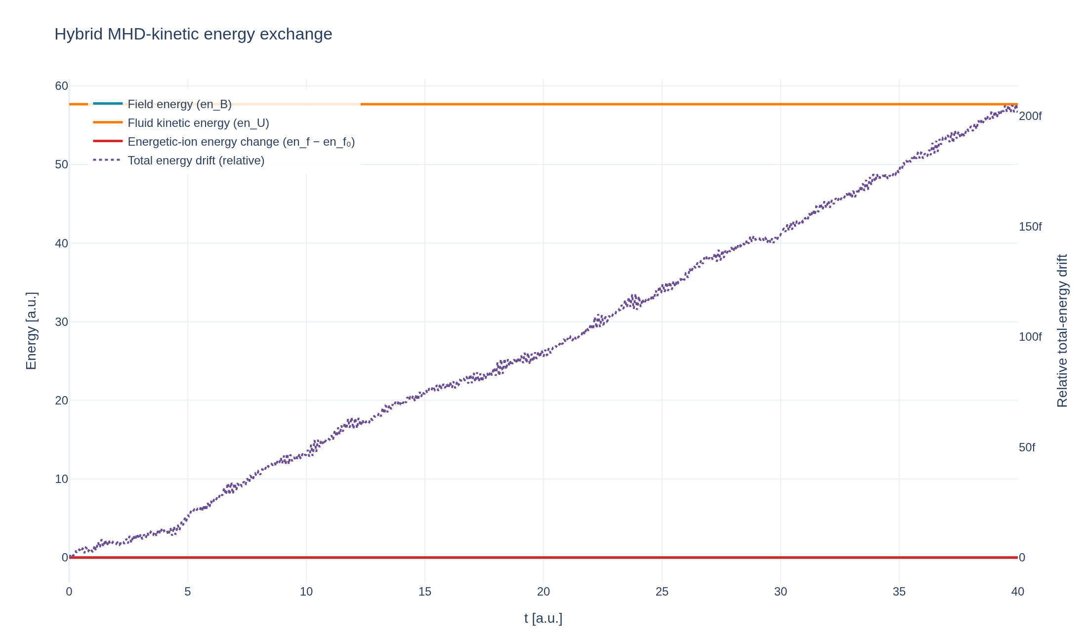

Actual output from the script below. The field (en_B), fluid (en_U) and energetic-ion (en_f) energies all move as the two subsystems exchange energy through the coupling term, while the total stays conserved to within 0.0e+0 relative drift — the defining property of a structure-preserving hybrid scheme, whether or not the configuration is unstable.

Physical problem

Two-way kinetic-MHD coupling

A bulk MHD fluid carries a shear-Alfvén wave along a uniform background field, while a population of energetic ions — too dilute to treat fluidly — is evolved kinetically with Struphy's 6D Vlasov pusher. The two are coupled through a pressure term: the ions feel the wave's fields, and their perpendicular pressure feeds back onto the fluid momentum equation. Struphy's structure-preserving discretization conserves the combined energy of both subsystems exactly, letting energy move freely between the kinetic and fluid pictures without any spurious gain or loss.

PDEs solved by model:

MHD continuity:

\frac{\partial ρ ~}{\partial t} + \nabla \cdot (ρ_{0} U ~) = 0

MHD momentum:

ρ_{0} \frac{\partial U ~}{\partial t} + \nabla p ~ + \frac{A _{h}}{A _{b}} \nabla \cdot P ~_{h, ⊥} = (\nabla \times B ~) \times B_{0} + J_{0} \times B ~

J_{0} = \nabla \times B_{0}

MHD pressure:

\frac{\partial p ~}{\partial t} + \nabla \cdot (p_{0} U ~) + \frac{2}{3} p_{0} \nabla \cdot U ~ = 0

MHD induction:

\frac{\partial B ~}{\partial t} - \nabla \times (U ~ \times B_{0}) = 0

Energetic-particle Vlasov equation:

\frac{\partial f _{h}}{\partial t} + (v + U ~_{⊥}) \cdot \nabla f_{h} + [\frac{1}{ϵ} v \times (B_{0} + B ~) - \nabla U ~_{⊥} \cdot v] \cdot \frac{\partial f _{h}}{\partial v} = 0

Perpendicular pressure tensor:

P ~_{h, ⊥} = \int v_{⊥} v_{⊥}^{⊤} f_{h} d v

Model: LinearMHDVlasovPC
Domain: Cuboid (r3=20)
Grid: 1 × 1 × 32
FEEC degree: 1 × 1 × 3
Integrator: Analytic
Evolution: 2,000 steps
Visualization: Plotly

Performance

Where the time goes

Download profile .h5

Struphy's built-in scope-profiler instruments every propagator, pusher and solver call — these are the real per-call timings from the run above, rendered live from its data.

Durations

Gantt (rank 0)

Region statistics

Region	Count	Avg (s)	Min (s)	Max (s)	Total (s)

Complete source

Run the simulation

Download .py

Requires Struphy 3.2 with compiled kernels and Plotly. Run struphy compile once, then execute python hybrid-alfven-ion-coupling.py.

"""Hybrid MHD-kinetic energy exchange with Struphy's LinearMHDVlasovPC model.

A population of energetic ions, drifting close to the Alfvén speed along a
uniform background field, is evolved together with a linear-MHD shear-Alfvén
wave via the pressure-coupling scheme. The two subsystems continuously trade
energy back and forth through the coupling term while the discretization
conserves the total -- the defining property of a structure-preserving hybrid
scheme.

Requires Struphy 3.2 with compiled kernels (`struphy compile`).
"""

import json
import os
import shutil
from pathlib import Path

import h5py
import numpy as np
import plotly.graph_objects as go

from struphy import (
    BoundaryParameters,
    DerhamOptions,
    EnvironmentOptions,
    FieldsBackground,
    LoadingParameters,
    SavingParameters,
    Simulation,
    SortingParameters,
    Time,
    WeightsParameters,
    domains,
    equils,
    grids,
    maxwellians,
    perturbations,
)
from struphy.models import LinearMHDVlasovPC

model = LinearMHDVlasovPC()
model.em_fields.b_field.save_data = True

# A periodic domain aligned with the background field, so energetic ions can
# free-stream along B0 and resonate with the Alfvén wave.
domain = domains.Cuboid(r3=20.0)
equil = equils.HomogenSlab(B0z=1.0, n0=1.0, beta=0.1)
grid = grids.TensorProductGrid(num_elements=(1, 1, 32))
derham_opts = DerhamOptions(degree=(1, 1, 3))
time_opts = Time(dt=0.02, Tend=40.0)

# A modest population of energetic ions, sorted into boxes for efficient
# accumulation of the pressure-coupling term onto the field grid.
model.energetic_ions.set_markers(
    loading_params=LoadingParameters(Np=8000, seed=1),
    weights_params=WeightsParameters(),
    boundary_params=BoundaryParameters(),
    sorting_params=SortingParameters(boxes_per_dim=(1, 1, 8), do_sort=True),
    saving_params=SavingParameters(),
)

model.propagators.push_eta_pc.options = model.propagators.push_eta_pc.Options()
model.propagators.push_vxb.options = model.propagators.push_vxb.Options()
model.propagators.pc6d.options = model.propagators.pc6d.Options()
model.propagators.shearalfven.options = model.propagators.shearalfven.Options()
model.propagators.magnetosonic.options = model.propagators.magnetosonic.Options()

# A small-amplitude shear-Alfvén seed, and energetic ions drifting near the
# resonant parallel velocity u3 = v_A = 1 with a finite thermal spread.
model.mhd.velocity.add_background(FieldsBackground())
model.mhd.velocity.add_perturbation(perturbations.Noise(amp=1e-3, comp=0, seed=42))
model.energetic_ions.var.add_background(
    maxwellians.Maxwellian3D(n=(0.1, None), u3=(1.0, None), vth3=(0.3, None)),
)

env = EnvironmentOptions(
    out_folders="struphy_gallery_runs",
    sim_folder="hybrid_alfven_ion_coupling",
)
sim = Simulation(
    model=model,
    name="Hybrid MHD-kinetic energy exchange",
    description=(
        "Energetic ions drifting near the Alfvén speed exchange energy with a "
        "shear-Alfvén wave through Struphy’s pressure-coupling scheme, while "
        "the total energy stays conserved."
    ),
    env=env,
    time_opts=time_opts,
    domain=domain,
    equil=equil,
    grid=grid,
    derham_opts=derham_opts,
)

if __name__ == "__main__":
    # scope-profiler is built into Struphy: this instruments every propagator,
    # pusher and solver call during the run and writes a timing HDF5 file.
    sim.run(profiling_activated=True)

    # LinearMHDVlasovPC tracks each subsystem's energy as a scalar every step:
    # en_B/en_U (field/fluid), en_f (kinetic energetic ions), en_tot (total).
    with h5py.File(os.path.join(env.path_out, "data", "data_proc0.hdf5"), "r") as f:
        time = np.asarray(f["time"]["value"])
        en_B = np.asarray(f["scalar"]["en_B"])
        en_U = np.asarray(f["scalar"]["en_U"])
        en_f = np.asarray(f["scalar"]["en_f"])
        en_tot = np.asarray(f["scalar"]["en_tot"])

    relative_drift = float(np.max(np.abs(en_tot - en_tot[0]) / en_tot[0]))
    print(f"Max relative drift in total energy (should be ~0): {relative_drift:.2e}")

    figure = go.Figure(
        data=[
            go.Scatter(x=time, y=en_B, mode="lines", name="Field energy (en_B)", line={"color": "#168aad", "width": 2.5}),
            go.Scatter(x=time, y=en_U, mode="lines", name="Fluid kinetic energy (en_U)", line={"color": "#f77f00", "width": 2.5}),
            go.Scatter(x=time, y=en_f - en_f[0], mode="lines", name="Energetic-ion energy change (en_f − en_f₀)", line={"color": "#d62828", "width": 2.5}),
            go.Scatter(
                x=time,
                y=(en_tot - en_tot[0]) / en_tot[0],
                mode="lines",
                name="Total energy drift (relative)",
                line={"color": "#6a4c93", "width": 2, "dash": "dot"},
                yaxis="y2",
            ),
        ],
    )
    figure.update_layout(
        title="Hybrid MHD-kinetic energy exchange",
        xaxis_title="t [a.u.]",
        yaxis_title="Energy [a.u.]",
        yaxis2={
            "title": "Relative total-energy drift",
            "overlaying": "y",
            "side": "right",
            "showgrid": False,
        },
        template="plotly_white",
        autosize=True,
        legend={"x": 0.02, "y": 0.98, "bgcolor": "rgba(255,255,255,0.82)"},
        margin={"l": 70, "r": 70, "t": 80, "b": 60},
    )

    png_path = Path("hybrid-alfven-ion-coupling.png")
    html_path = Path("hybrid-alfven-ion-coupling.html")
    figure.write_image(png_path, width=1100, height=650, scale=2)
    figure.write_html(
        html_path,
        include_plotlyjs="cdn",
        default_width="100%",
        default_height="100%",
        config={"responsive": True, "displaylogo": False},
    )
    print(f"Saved {png_path.resolve()}")
    print(f"Saved {html_path.resolve()}")

    # Export scope-profiler's plot-data JSON (durations, gantt, region
    # statistics) via its Python API, so the example page can render native
    # Plotly figures from the real run above -- not a separate report.
    from scope_profiler import plot_durations, plot_gantt, read_h5, write_region_statistics_json

    profile_reader = read_h5(sim.profiling_filepath)
    profile_h5_path = Path("hybrid-alfven-ion-coupling-profile.h5")
    shutil.copyfile(sim.profiling_filepath, profile_h5_path)

    durations_path = Path("hybrid-alfven-ion-coupling-durations.json")
    plot_durations(
        [profile_reader],
        ranks=[0],
        metrics=("total", "avg"),
        sort_by="total",
        stack_children=True,
        data_filepath=durations_path,
        data_format="json",
        verbose=False,
    )
    durations_payload = json.loads(durations_path.read_text())
    durations_payload["bars"] = [bar for bar in durations_payload["bars"] if bar["value_seconds"]]
    durations_path.write_text(json.dumps(durations_payload))

    gantt_path = Path("hybrid-alfven-ion-coupling-gantt.json")
    region_stats_path = Path("hybrid-alfven-ion-coupling-region-stats.json")
    plot_gantt([profile_reader], ranks=[0], data_filepath=gantt_path, data_format="json", verbose=False)
    write_region_statistics_json([profile_reader], region_stats_path, ranks=[0])

    GANTT_MAX_INTERVALS = 5000
    gantt_payload = json.loads(gantt_path.read_text())
    if len(gantt_payload["intervals"]) > GANTT_MAX_INTERVALS:
        gantt_payload["intervals"] = sorted(gantt_payload["intervals"], key=lambda c: c["start_seconds"])[:GANTT_MAX_INTERVALS]
        gantt_path.write_text(json.dumps(gantt_payload))
    print(f"Saved {profile_h5_path.resolve()}")
    print(f"Saved {durations_path.resolve()}, {gantt_path.resolve()}, {region_stats_path.resolve()}")

    metadata_path = Path("hybrid-alfven-ion-coupling.metadata.json")
    metadata = json.loads(metadata_path.read_text()) if metadata_path.exists() else {}
    metadata["relativeTotalEnergyDrift"] = relative_drift
    metadata["profilingData"] = "/examples/hybrid-alfven-ion-coupling-profile.h5"
    metadata["profilingDurations"] = "/examples/hybrid-alfven-ion-coupling-durations.json"
    metadata["profilingGantt"] = "/examples/hybrid-alfven-ion-coupling-gantt.json"
    metadata["profilingRegionStats"] = "/examples/hybrid-alfven-ion-coupling-region-stats.json"
    metadata_path.write_text(json.dumps(metadata, indent=2, ensure_ascii=False))
    print(f"Saved {metadata_path.resolve()}")

Uses Struphy's LinearMHDVlasovPC model, coupling linearized MHD to a 6D kinetic energetic-ion species via the pressure-coupling scheme. See the post-processing guide for more ways to inspect the result.