LinearMHD · MHD waves
MHD waves in a magnetized slab
Broadband noise excites the shear Alfvén wave and the slow and fast magnetosonic waves of a uniform, obliquely magnetized plasma. The power spectra of the velocity and the pressure show the three branches, and their fitted speeds are compared with the exact ideal-MHD values.
Run the simulation ↓← All examples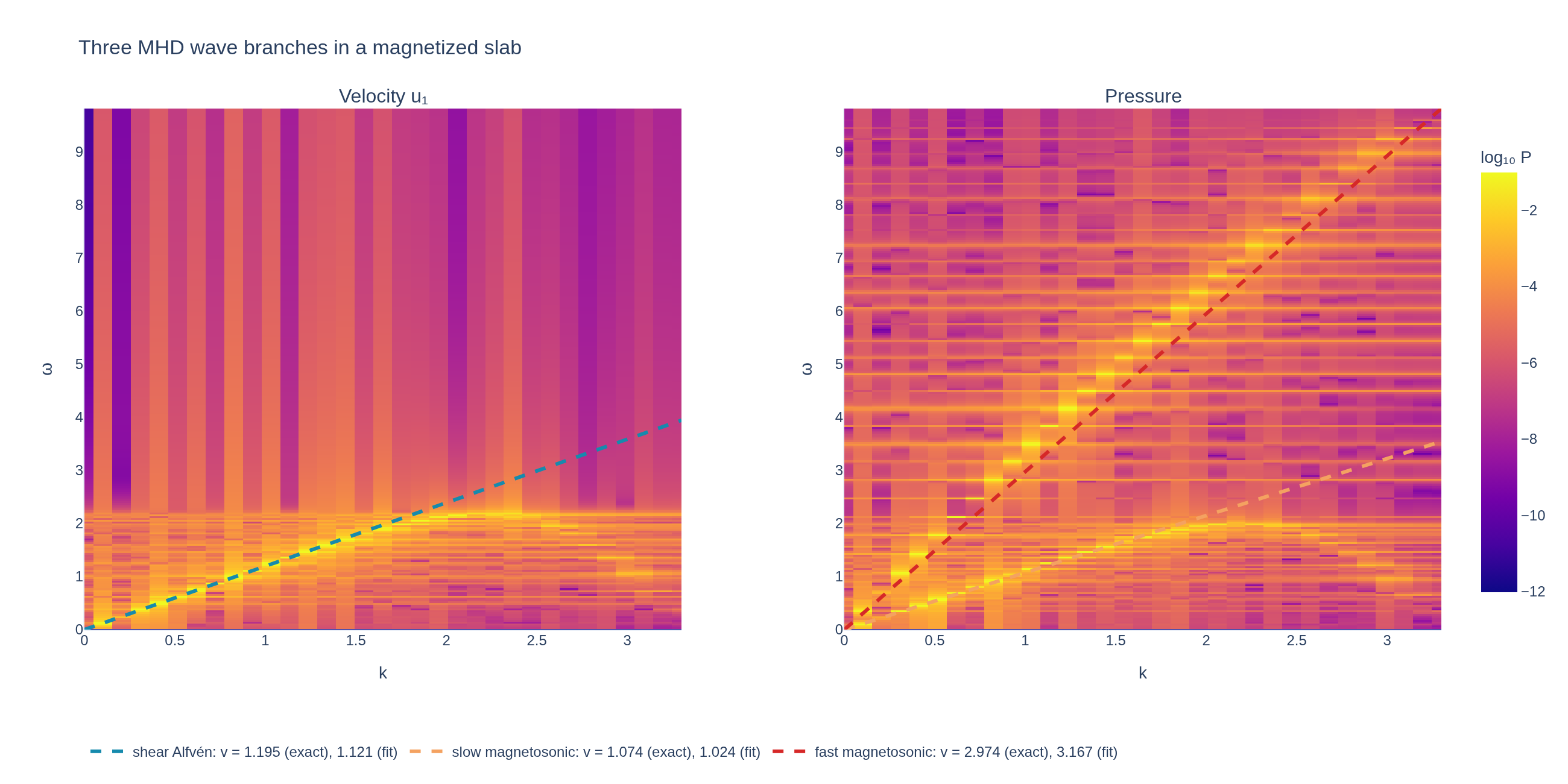
Physical problem
Three waves from one noise spectrum
Broadband noise excites the shear Alfvén wave and the slow and fast magnetosonic waves of a uniform, obliquely magnetized plasma. The power spectra of the velocity and the pressure show the three branches, and their fitted speeds are compared with the exact ideal-MHD values.
PDEs solved by model:
Continuity (mass conservation):
Momentum (Lorentz force):
Energy (adiabatic process):
Induction (Faraday's law):
- Model
- LinearMHD
- Domain
- Cuboid (r3=60)
- Grid
- 1 × 1 × 64
- FEEC degree
- 1 × 1 × 3
- Integrator
- Implicit
- Evolution
- 1,200 steps
- Visualization
- Plotly
Performance
Profiling
Struphy's built-in scope-profiler instruments every propagator, pusher and solver call — these are the real per-call timings from the run above.
Gantt (rank 0)
Region statistics
| Region | Count | Avg (s) | Min (s) | Max (s) | Total (s) |
|---|
Complete source
Run the simulation
Requires Struphy with compiled kernels and Plotly. Run struphy compile once, then execute python mhd-slab-waves.py.
"""The three MHD wave branches of a magnetized slab, with Struphy's LinearMHD model.

A uniform plasma in an oblique magnetic field carries three waves along z: the shear Alfvén wave, and
the slow and fast magnetosonic waves. Broadband noise in the velocity excites all of them at once. The
(k, omega) power spectrum of the velocity shows the Alfvén branch, that of the pressure the two
magnetosonic branches, and the speeds fitted to them are compared with the exact ideal-MHD values.

Adapted from Struphy's tutorial (tutorials/tutorial_linear_mhd_slab_waves_1d.ipynb).

Requires Struphy 3.3 with compiled kernels (`struphy compile`).
"""

import numpy as np
import plotly.graph_objects as go

from struphy import DerhamOptions, EnvironmentOptions, Simulation, Time, domains, equils, grids, perturbations
from struphy.diagnostics.diagn_tools import power_spectrum_2d
from struphy.models import LinearMHD

# The background: B0 = (0, 1, 1), density 0.7 and a plasma beta of 3 (thermal over magnetic pressure).
B0x, B0y, B0z = 0.0, 1.0, 1.0
n0, beta, gamma = 0.7, 3.0, 5.0 / 3.0
B_squared = B0x**2 + B0y**2 + B0z**2
p0 = beta * B_squared / 2.0

# Ideal-MHD wave speeds along z: the shear Alfvén wave, and the slow and fast magnetosonic waves.
alfven_speed = np.sqrt(B_squared / n0)
sound_speed = np.sqrt(gamma * p0 / n0)
delta = 4 * B0z**2 * sound_speed**2 * alfven_speed**2 / ((sound_speed**2 + alfven_speed**2) ** 2 * B_squared)
exact_speeds = {
    "alfven": alfven_speed * B0z / np.sqrt(B_squared),
    "slow": np.sqrt(0.5 * (sound_speed**2 + alfven_speed**2) * (1.0 - np.sqrt(1.0 - delta))),
    "fast": np.sqrt(0.5 * (sound_speed**2 + alfven_speed**2) * (1.0 + np.sqrt(1.0 - delta))),
}

model = LinearMHD()
model.propagators.shear_alf.options = model.propagators.shear_alf.Options(algo="implicit")

# Broadband noise in all three velocity components, so that every branch is excited.
for component in range(3):
    model.mhd.velocity.add_perturbation(perturbations.Noise(amp=0.1, comp=component, seed=123))

domain = domains.Cuboid(r3=60.0)
grid = grids.TensorProductGrid(num_elements=(1, 1, 64))
derham_opts = DerhamOptions(degree=(1, 1, 3))
equil = equils.HomogenSlab(B0x=B0x, B0y=B0y, B0z=B0z, beta=beta, n0=n0)
time_opts = Time(dt=0.15, Tend=180.0)

env = EnvironmentOptions(out_folders="struphy_gallery_runs", sim_folder="mhd_slab_waves")
sim = Simulation(
    model=model,
    name="MHD waves in a magnetized slab",
    description=(
        "Broadband noise excites the shear Alfvén wave and the slow and fast magnetosonic waves of a "
        "uniform, obliquely magnetized plasma. The power spectra of the velocity and the pressure show "
        "the three branches, and their fitted speeds are compared with the exact ideal-MHD values."
    ),
    env=env,
    time_opts=time_opts,
    domain=domain,
    equil=equil,
    grid=grid,
    derham_opts=derham_opts,
)


if __name__ == "__main__":
    from plotly.subplots import make_subplots

    from _gallery import export_profiling, merge_metadata, save_figure

    output = sim.run(profiling_activated=True)
    output.pproc(physical=True)

    disp_params = {"B0x": B0x, "B0y": B0y, "B0z": B0z, "p0": p0, "n0": n0, "gamma": gamma}
    common = {"slice_at": [0, 0, None], "physical": True, "do_plot": False, "extr_order": 10}
    omega_u, k_u, spectrum_u, fit_u = power_spectrum_2d(
        output.fields.mhd.velocity,
        component=0,
        fit_branches=1,
        noise_level=0.5,
        fit_degree=(1,),
        **common,
    )
    omega_p, k_p, spectrum_p, fit_p = power_spectrum_2d(
        output.fields.mhd.pressure,
        component=0,
        fit_branches=2,
        noise_level=0.4,
        fit_degree=(1, 1),
        **common,
    )
    measured_speeds = {
        "alfven": float(fit_u[0][0]),
        "slow": float(fit_p[0][0]),
        "fast": float(fit_p[1][0]),
    }
    for branch, exact in exact_speeds.items():
        print(f"{branch}: measured {measured_speeds[branch]:.4f}, exact {exact:.4f}")
    if not all(np.isfinite(v) for v in measured_speeds.values()):
        raise RuntimeError("A wave branch could not be fitted")

    def log_power(spectrum):
        power = np.asarray(spectrum) ** 2
        return np.log10(np.clip(power / power.max(), 1e-15, None))

    k_top = float(min(k_u[-1], k_p[-1]))
    colors = {"alfven": "#168aad", "slow": "#f4a261", "fast": "#d62828"}
    labels = {"alfven": "shear Alfvén", "slow": "slow magnetosonic", "fast": "fast magnetosonic"}
    panels = (
        ("Velocity u₁", omega_u, k_u, spectrum_u, ("alfven",)),
        ("Pressure", omega_p, k_p, spectrum_p, ("slow", "fast")),
    )
    figure = make_subplots(rows=1, cols=2, subplot_titles=[panel[0] for panel in panels], horizontal_spacing=0.12)
    for column, (_, omega, k, spectrum, branches) in enumerate(panels, start=1):
        figure.add_trace(
            go.Heatmap(
                x=np.asarray(k), y=np.asarray(omega), z=log_power(spectrum), zmin=-12, zmax=-1,
                colorscale="Plasma", showscale=column == 2,
                colorbar={"title": {"text": "log₁₀ P"}, "len": 0.9},
                hovertemplate="k=%{x:.3f}<br>ω=%{y:.3f}<br>log₁₀ P=%{z:.2f}<extra></extra>",
            ),
            row=1, col=column,
        )
        for branch in branches:
            figure.add_trace(
                go.Scatter(
                    x=[0, k_top], y=[0, exact_speeds[branch] * k_top], mode="lines",
                    name=f"{labels[branch]}: v = {exact_speeds[branch]:.3f} (exact), "
                         f"{measured_speeds[branch]:.3f} (fit)",
                    line={"color": colors[branch], "width": 3, "dash": "dash"}, legendgroup=branch,
                ),
                row=1, col=column,
            )
        figure.update_xaxes(title_text="k", range=[0, k_top], row=1, col=column)
        figure.update_yaxes(title_text="ω", range=[0, exact_speeds["fast"] * k_top], row=1, col=column)
    figure.update_layout(
        title="Three MHD wave branches in a magnetized slab", template="plotly_white",
        legend={"orientation": "h", "y": -0.2}, margin={"l": 70, "r": 40, "t": 90, "b": 110},
    )
    save_figure(figure, "mhd-slab-waves", width=1300, height=650)

    merge_metadata(
        "mhd-slab-waves",
        measuredAlfvenSpeed=measured_speeds["alfven"], exactAlfvenSpeed=float(exact_speeds["alfven"]),
        measuredSlowSpeed=measured_speeds["slow"], exactSlowSpeed=float(exact_speeds["slow"]),
        measuredFastSpeed=measured_speeds["fast"], exactFastSpeed=float(exact_speeds["fast"]),
        **export_profiling(sim, "mhd-slab-waves"),
    )
See the post-processing guide for more ways to inspect the result.