Vlasov particle orbits in a tokamak

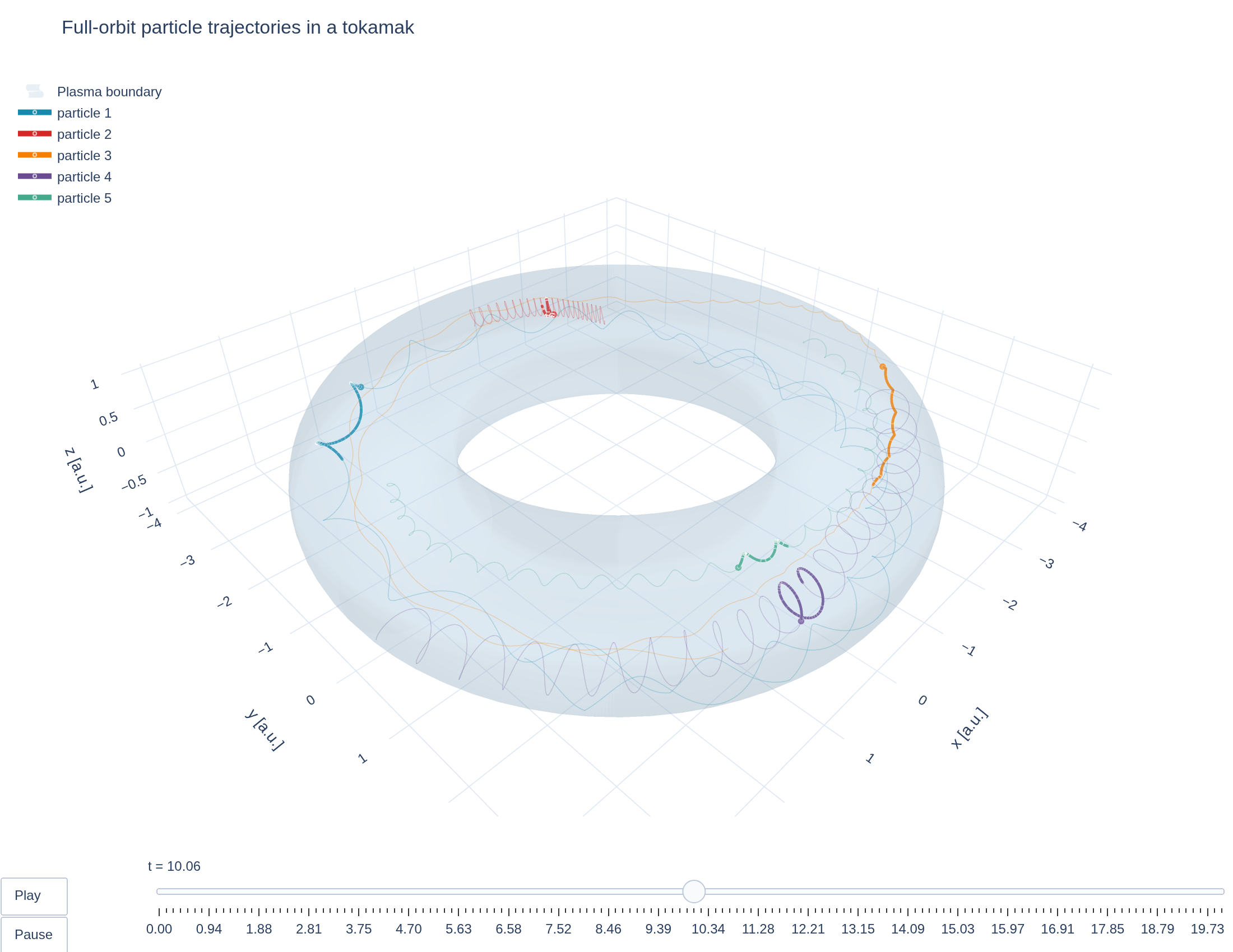
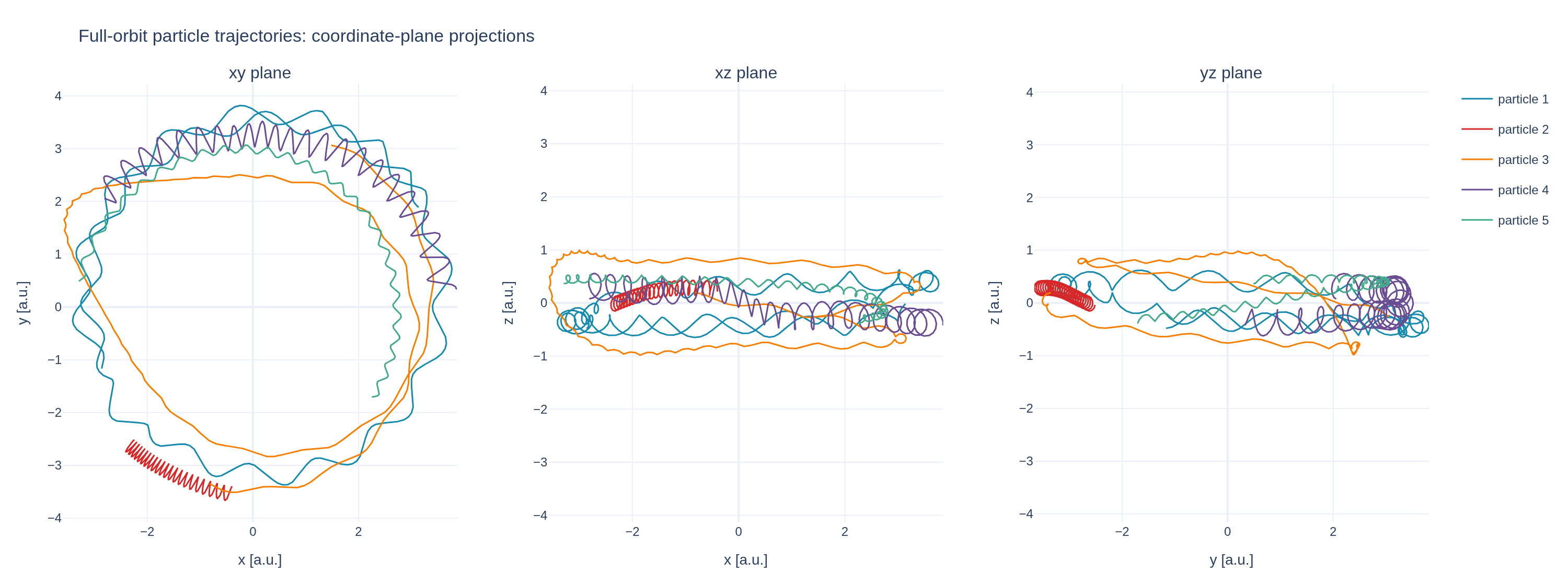
"""Trace full-orbit test particles through a tokamak's magnetic field.

A handful of markers are seeded from a Maxwellian and pushed with Struphy's
full-orbit (Vlasov) pusher through the static magnetic field of an analytic
tokamak equilibrium, on a flux-aligned `Tokamak` domain. No fields are solved
self-consistently -- this traces single-particle motion in a fixed background
field, so each particle should gyrate around a field line while it circulates
(or bounces) through the torus, conserving its speed exactly.

Requires Struphy 3.2 with compiled kernels (`struphy compile`).
"""

import json
from pathlib import Path

import numpy as np
import plotly.graph_objects as go

from struphy import (
    DerhamOptions,
    EnvironmentOptions,
    Simulation,
    Time,
    domains,
    grids,
)
from struphy.fields_background import equils
from struphy.kinetic_background import maxwellians
from struphy.models import Vlasov
from struphy.pic.base import BoundaryParameters, LoadingParameters, SavingParameters

model = Vlasov(charge_number=1, mass_number=1.0)
model.kinetic_ions.var.add_background(maxwellians.Maxwellian3D())

# Load a small population; only a handful of markers have their full orbit saved.
# eta1 is the radial flux coordinate on this domain, so it must reflect at the
# plasma edge/axis rather than wrap periodically like the two angular
# coordinates (eta2, eta3) -- periodic in eta1 would teleport a particle from
# the outer edge back to the magnetic axis. The tracked markers start at a
# modest radius (rather than anywhere in [0, 1]) so their orbits stay clear of
# that reflecting boundary for most of the run.
n_tracked = 5
tracked_start = tuple((0.35, None, None, None, None, None) for _ in range(n_tracked))
model.kinetic_ions.set_markers(
    loading_params=LoadingParameters(Np=300, seed=7, specific_markers=tracked_start),
    saving_params=SavingParameters(n_markers=n_tracked),
    boundary_params=BoundaryParameters(bc=("reflect", "periodic", "periodic")),
)

# A flux-aligned tokamak domain, built by field-line tracing an analytic
# axisymmetric MHD equilibrium. A stronger-than-default field (B0) shrinks the
# Larmor radius, so gyration shows up as tight loops on top of the smooth
# guiding-center motion instead of dominating it.
equil = equils.AdhocTorus(B0=8.0)
domain = domains.Tokamak(equilibrium=equil, num_elements=(4, 16), degree=(2, 3))
grid = grids.TensorProductGrid(num_elements=(8, 12, 4))
derham_opts = DerhamOptions(degree=(1, 2, 1))
time_opts = Time(dt=0.005, Tend=20.0)

env = EnvironmentOptions(
    out_folders="struphy_gallery_runs",
    sim_folder="vlasov_tokamak",
)
sim = Simulation(
    model=model,
    name="Vlasov particle orbits in a tokamak",
    description=(
        "Trace full-orbit test particles through a tokamak’s magnetic field "
        "and watch them gyrate around field lines while circulating -- or "
        "bouncing -- through the torus."
    ),
    env=env,
    time_opts=time_opts,
    domain=domain,
    equil=equil,
    grid=grid,
    derham_opts=derham_opts,
)

if __name__ == "__main__":
    sim.run()
    sim.pproc(create_vtk=False)
    sim.load_plotting_data()

    # (time, particle, [x, y, z, v1, v2, v3, weight, id]) in physical coordinates.
    orbits = np.asarray(sim.orbits.kinetic_ions)

    # A magnetic field alone does no work, so each particle's speed should be
    # conserved -- a genuine accuracy check on the pusher, not just a demo.
    speed = np.linalg.norm(orbits[:, :, 3:6], axis=2)
    max_relative_speed_drift = float(np.max(np.abs(speed - speed[0]) / speed[0]))
    print(f"Max relative drift in particle speed (should be ~0): {max_relative_speed_drift:.5f}")

    # The plasma boundary (outer flux surface), for visual context around the orbits.
    boundary_x, boundary_y, boundary_z = domain.outer_boundary_mesh(n2=40, n3=80)

    figure = go.Figure()
    figure.add_trace(
        go.Surface(
            x=boundary_x,
            y=boundary_y,
            z=boundary_z,
            colorscale=[[0, "#a9c4d8"], [1, "#a9c4d8"]],
            showscale=False,
            opacity=0.25,
            hoverinfo="skip",
            name="Plasma boundary",
            showlegend=True,
        ),
    )
    palette = ["#168aad", "#d62828", "#f77f00", "#6a4c93", "#43aa8b"]
    for p in range(orbits.shape[1]):
        figure.add_trace(
            go.Scatter3d(
                x=orbits[:, p, 0],
                y=orbits[:, p, 1],
                z=orbits[:, p, 2],
                mode="lines",
                line={"width": 4, "color": palette[p % len(palette)]},
                name=f"particle {p + 1}",
            ),
        )
    figure.update_layout(
        title="Full-orbit particle trajectories in a tokamak",
        scene={
            "xaxis_title": "x [a.u.]",
            "yaxis_title": "y [a.u.]",
            "zaxis_title": "z [a.u.]",
            "aspectmode": "data",
        },
        template="plotly_white",
        margin={"l": 0, "r": 0, "t": 60, "b": 0},
        legend={"x": 0.01, "y": 0.99, "bgcolor": "rgba(255,255,255,0.75)"},
    )

    png_path = Path("vlasov-tokamak.png")
    html_path = Path("vlasov-tokamak.html")
    figure.write_image(png_path, width=1100, height=850, scale=2)
    figure.write_html(
        html_path,
        include_plotlyjs="cdn",
        default_width="100%",
        default_height="100%",
        config={"responsive": True, "displaylogo": False},
    )
    print(f"Saved {png_path.resolve()}")
    print(f"Saved {html_path.resolve()}")

    metadata_path = Path("vlasov-tokamak.metadata.json")
    metadata = json.loads(metadata_path.read_text()) if metadata_path.exists() else {}
    metadata["maxRelativeSpeedDrift"] = max_relative_speed_drift
    metadata["trackedParticles"] = n_tracked
    metadata_path.write_text(json.dumps(metadata, indent=2, ensure_ascii=False))
    print(f"Saved {metadata_path.resolve()}")