Kinetic model

Vlasov

Vlasov equation for a single species in a static background magnetic field.

← All models Reference documentation ↗

Overview

Vlasov is the simplest kinetic test-particle model in the 6D hierarchy.

It evolves particles in a static magnetic background without electric or magnetic self-consistency.

Use cases

This model is appropriate for:

test-particle motion in prescribed magnetic fields
verification of the Boris-like VxB and PushEta splitting
reduced kinetic transport studies without field feedback

Governing equations

PDEs solved by model:

Vlasov equation:

\frac{\partial f}{\partial t} + v \cdot \nabla f + (v \times B_{0}) \cdot \frac{\partial f}{\partial v} = 0

Normalization

The characteristic speed is the cyclotron scale

v^= Ω^_{c} x^.

Discretization

Time integration is performed by the following propagators (in sequence):

Diagnostics

The following scalars are tracked during simulation:

Particle kinetic energy: kinetic_energy

Examples

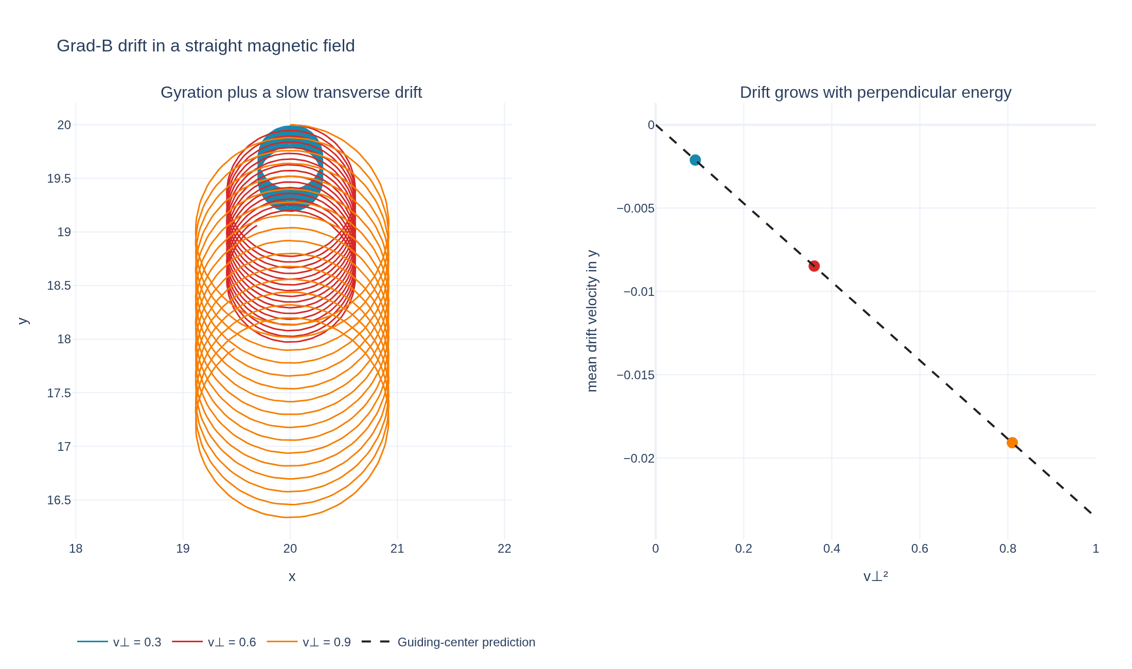
Grad-B drift of charged particles

Charged particles gyrate more tightly on the stronger-field side of an orbit, producing a drift perpendicular to both the magnetic field and its gradient. Three test ions demonstrate how the drift grows with perpendicular kinetic energy. The magnetic field is externally prescribed; its straight field lines exclude curvature drift. Here $\mathbf{B}(x)=[1+0.3\sin(2\pi x/40)]\mathbf{e}_z,$ and the ions start at $(20,20,20)$ with $\mathbf{v}_0=(v_\perp,0,0)$ , $v_\perp\in\{0.3,0.6,0.9\}$ and $q/m=1$ . Their measured drift is compared with the guiding-center approximation $v_{\nabla B,y}=v_\perp^2 B'/(2B^2)$ .

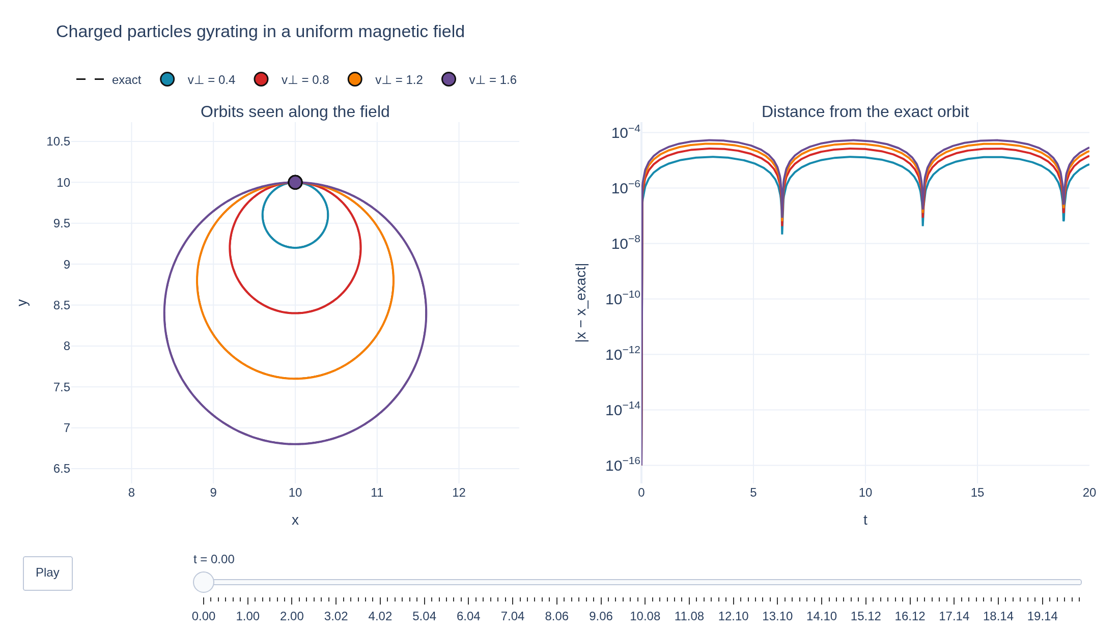
Gyromotion in a uniform magnetic field

Test particles with different perpendicular speeds circle a uniform magnetic field at the same gyrofrequency, on circles whose Larmor radius grows with the perpendicular speed, while they stream freely along the field. Struphy's full-orbit pusher is compared with the exact helices. All four particles start at $\mathbf{x}_0=(10,10,2)$ in $\mathbf{B}_0=\mathbf{e}_z$ , with $\mathbf{v}_{0,j}=(0.4j,0,0.2j),\qquad j=1,2,3,4.$ Their Larmor radii are $r_{L,j}=v_{\perp,j}/\Omega_c$ , with normalized gyrofrequency $\Omega_c=1$ .

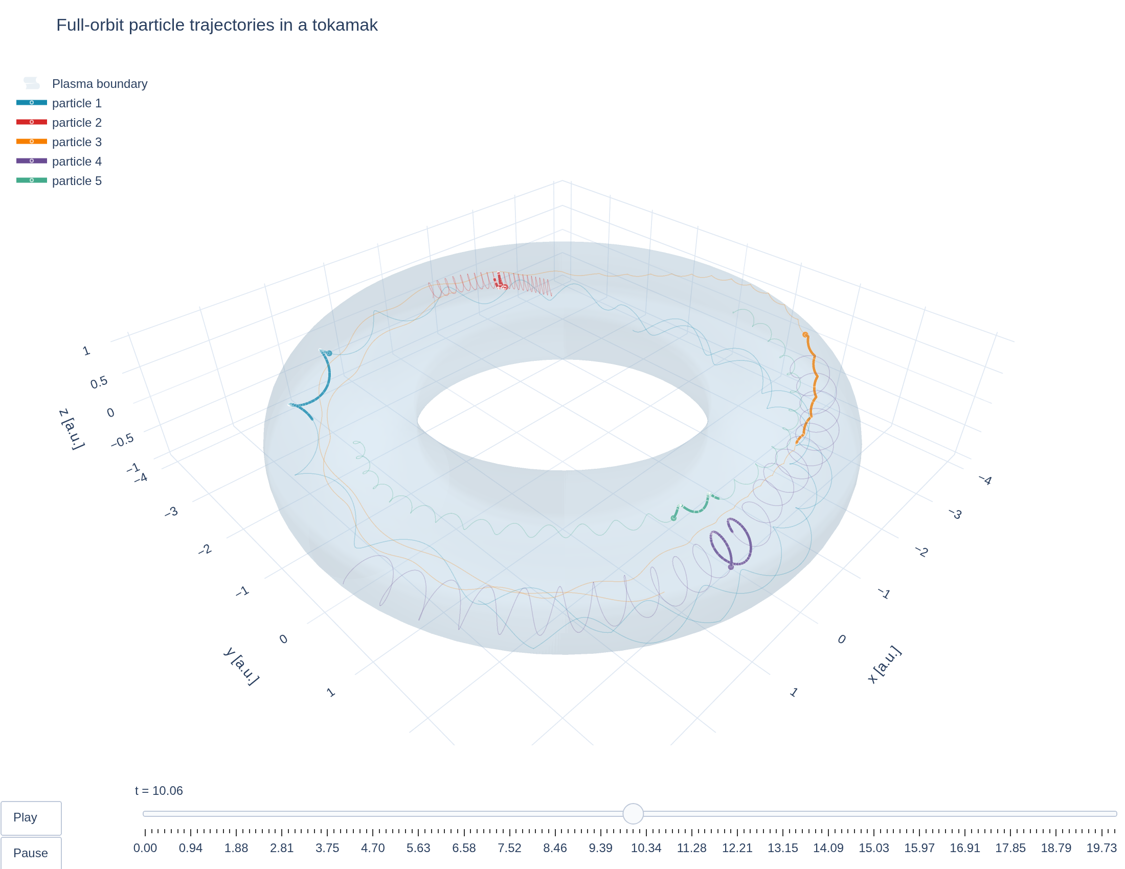
Vlasov particle orbits in a tokamak

Trace full-orbit test particles through a tokamak’s magnetic field and watch them gyrate around field lines while circulating -- or bouncing -- through the torus. Velocities are drawn from the unit-thermal-speed Maxwellian $f_0(\mathbf{v})=(2\pi)^{-3/2}e^{-|\mathbf{v}|^2/2}.$ The five tracked particles start at logical radius $\eta_1=0.35$ , with random angles, in an equilibrium with field parameter $B_0=8$ .