VlasovAmpereOneSpecies · Kinetic electrostatics
Weak Landau damping
A tiny electrostatic perturbation phase-mixes away in a collisionless plasma — the classic Landau-damping benchmark, compared here against the linear damping rate at wavenumber in normalized units. The initial Maxwellian has density zero mean velocity and thermal speed .
Loading interactive figure…
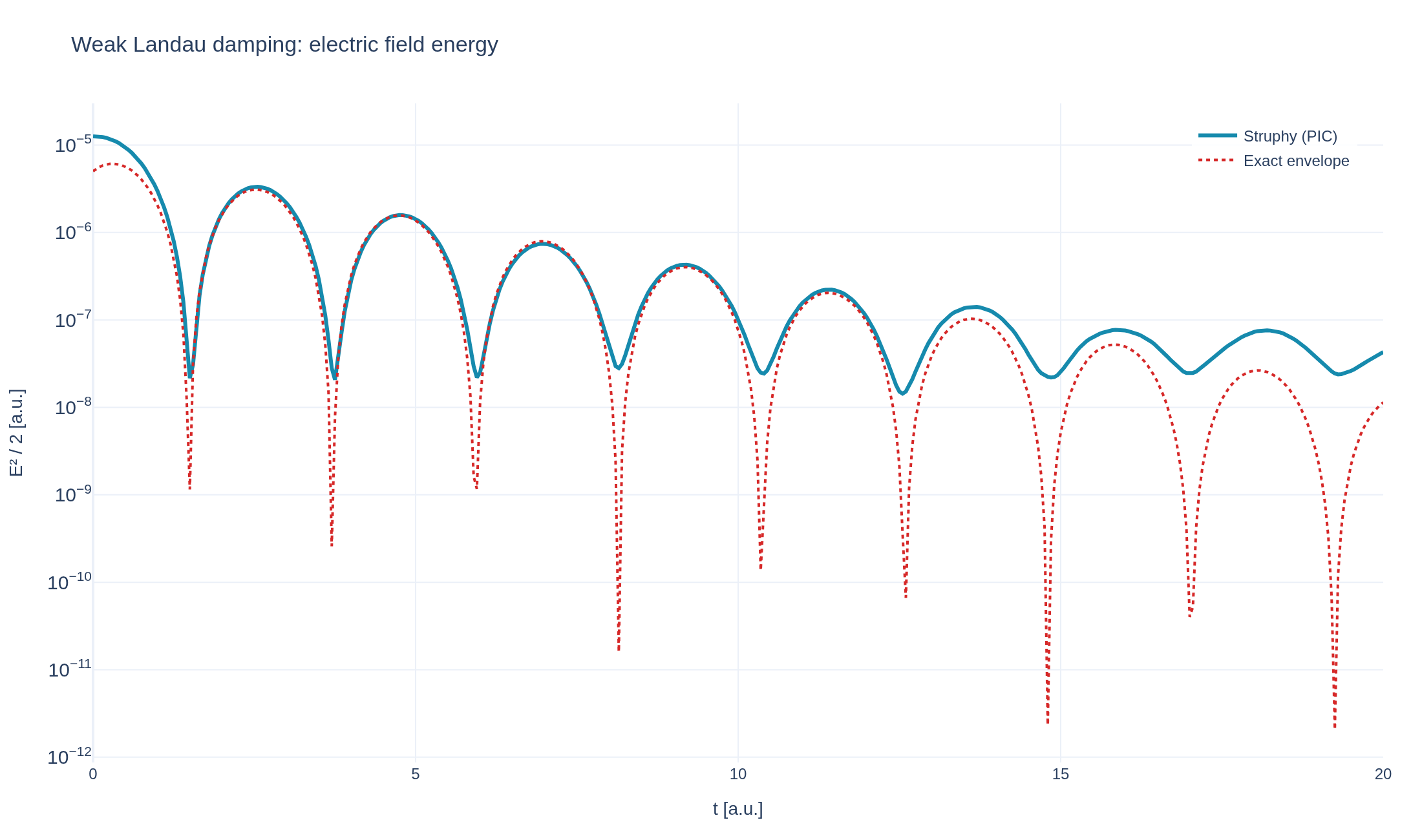
Loading interactive figure…
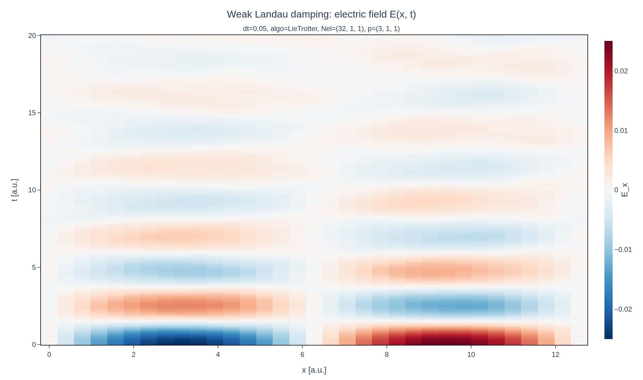
Physical problem
Phase mixing in a uniform plasma
PDEs solved by model:
Vlasov equation:
Ampère's law:
Initial Poisson equation: At , solve weakly for the electric potential :
Simulation geometry
Domain used in this run
The actual Cuboid geometry reconstructed from this run's metadata. Switch between the 3D view and physical-coordinate slices.
Domain
Cuboid
Mapping
Loading Cuboid…
Parameters
| Parameter | Value | Description |
|---|---|---|
| Loading parameters… | ||
Performance
Profiling
Struphy's built-in scope-profiler instruments every propagator, pusher and solver call — these are the real per-call timings from the run above.
Durations
Gantt (rank 0)
Region statistics
| Region | Count | Avg (s) | Min (s) | Max (s) | Total (s) |
|---|
Complete source
Simulation script
Run it locally
1. Install and compile
Use Python 3.10 or newer with Struphy's system prerequisites installed. Run these commands in your Python environment:
pip install "struphy[pproc]>=3.4.0"
pip install "plasma-plots[plotly]>=0.1.1"
struphy compile
PNG exports need Chrome or Chromium. If Chrome is not installed, run kaleido_get_chrome.
2. Run the script
Download the .py file above, open a terminal in its directory, then run:
python weak-landau-damping.pyFigures are saved in the current directory. Add --show to display them before saving.
"""Weak Landau damping: the canonical Vlasov-Ampère verification case.

A tiny electrostatic perturbation in a uniform, collisionless plasma damps
exponentially as particles phase-mix with the self-consistent field --
Landau damping. This benchmark validates the coupled Vlasov-Ampère PIC
discretization against the analytically known damping rate.

Adapted from Struphy's maintained example (examples/VlasovAmpereOneSpecies/weak_Landau_damping).

Install dependencies and compile the kernels (Python 3.10 or newer):

    pip install "struphy[pproc]>=3.4.0"
    pip install "plasma-plots[plotly]>=0.1.1"
    struphy compile

PNG exports require Chrome or Chromium. If Chrome is not installed, run:

    kaleido_get_chrome

Save this file and run it from the directory where you want the output:

    python weak-landau-damping.py

Figures are saved in the current directory; add --show to display them before saving.
"""

import argparse

import numpy as np

from struphy import (
    BoundaryParameters,
    DerhamOptions,
    EnvironmentOptions,
    LoadingParameters,
    SavingParameters,
    Simulation,
    SortingParameters,
    Time,
    WeightsParameters,
    domains,
    grids,
    maxwellians,
    perturbations,
)
from struphy.models import VlasovAmpereOneSpecies
from plasma_plots import save_figure

# A single small-amplitude cosine mode perturbs an otherwise uniform Maxwellian.
perturbation_amplitude = 0.001


def create_simulation() -> Simulation:
    model = VlasovAmpereOneSpecies(alpha=1.0, epsilon=-1.0, with_B0=False)
    model.em_fields.e_field.save_data = True

    # A periodic box of length 4*pi (k = 0.5), resolved by a single, low-degree element row.
    domain = domains.Cuboid(r1=12.56)
    grid = grids.TensorProductGrid(num_elements=(32, 1, 1))
    derham_opts = DerhamOptions(degree=(3, 1, 1))
    time_opts = Time(dt=0.05, Tend=20.0, split_algo="LieTrotter")

    # 1000 particles per cell, sorted into boxes for the control-variate weighting.
    model.kinetic_ions.set_markers(
        loading_params=LoadingParameters(ppc=1000),
        weights_params=WeightsParameters(control_variate=True),
        boundary_params=BoundaryParameters(),
        sorting_params=SortingParameters(boxes_per_dim=(16, 1, 1), do_sort=True),
        saving_params=SavingParameters(),
        bufsize=2.0,
    )

    model.propagators.push_eta.options = model.propagators.push_eta.Options()
    model.propagators.coupling_va.options = model.propagators.coupling_va.Options()
    model.initial_poisson.options = model.initial_poisson.Options(stab_mat="M0")
    background = maxwellians.Maxwellian3D(n=(1.0, None))
    model.kinetic_ions.var.add_background(background)
    perturbation = perturbations.ModesCos(amps=(perturbation_amplitude,), ls=(1,))
    model.kinetic_ions.var.add_initial_condition(maxwellians.Maxwellian3D(n=(1.0, perturbation)))

    env = EnvironmentOptions(
        out_folders="struphy_gallery_runs",
        sim_folder="weak_landau_damping",
    )
    sim = Simulation(
        model=model,
        name="Weak Landau damping",
        description=(
            "A tiny electrostatic perturbation phase-mixes away in a collisionless "
            "plasma — the classic Landau-damping benchmark, compared here against "
            r"the linear damping rate :math:`\gamma \approx -0.1533` at "
            r"wavenumber :math:`k \approx 0.5` in normalized units."
            r" The initial Maxwellian has density $$n(x,0)=1+10^{-3}\cos(2\pi x/L),\qquad L=12.56,$$"
            r" zero mean velocity and thermal speed :math:`v_{\mathrm{th}}=1`."
        ),
        env=env,
        time_opts=time_opts,
        domain=domain,
        grid=grid,
        derham_opts=derham_opts,
    )
    return sim


def pproc(sim: Simulation, show: bool = False):
    domain = sim.domain

    # The exact linear damping rate/frequency for k = 0.5 (Cuboid r1 = 4*pi),
    # from the Vlasov-Ampère dispersion relation (see the struphy verification test).
    def field_energy_exact(t):
        r, omega_r, omega_i, phi = 0.3677, 1.4156, -0.1533, 0.5362
        return (4 * perturbation_amplitude * r * np.exp(omega_i * t) * np.cos(omega_r * t - phi)) ** 2 * np.pi

    output = sim.output
    field_energy = output.scalars["electric_energy"]
    time = np.asarray(field_energy.t)

    # Fit the damping rate from the envelope maxima, for comparison with omega_i = -0.1533.
    # Only fit the clean exponential-decay region -- once the signal drops
    # below the discrete-particle noise floor (around t ~ 8 here), later
    # envelope maxima track PIC noise rather than the physical damping.
    measured_rate = field_energy.plasma.analysis.damping_rate(window=(None, 8.0), amplitude=True).rate
    print(f"Measured damping rate: {measured_rate:.4f} (exact: -0.1533)")

    figure = field_energy.plasma.plot.timeseries(
        logy=True,
        reference={"Exact envelope": (time, field_energy_exact(time))},
        title="Weak Landau damping: electric field energy",
        backend="plotly",
    )

    save_figure(figure, "weak-landau-damping", show=show)

    # The electric field along x, over time.
    output.pproc()
    electric_field = output.evaluate(
        "em_fields/e_field", eta1=np.linspace(0.0, 1.0, output.grid.num_elements[0] + 1), eta2=0.0, eta3=0.0,
        representation="1",
    ).isel(component=0)  # (t, eta1)
    space_time = electric_field.assign_coords(eta1=electric_field.eta1.values * domain.params["r1"]).plasma.plot.slice(
        x="eta1",
        y="t",
        symmetric=True,
        cmap="RdBu_r",
        title="Weak Landau damping: electric field E(x, t)",
        xlabel="x [a.u.]",
        ylabel="t [a.u.]",
        colorbar_label="E_x",
        backend="plotly",
    )
    save_figure(space_time, "weak-landau-damping-space-time", show=show)


if __name__ == "__main__":
    argparser = argparse.ArgumentParser(description="Run the weak landau damping example.")
    argparser.add_argument(
        "--pproc-only",
        action="store_true",
        help="Run post-processing on an existing simulation instead of running a new one.",
    )
    argparser.add_argument("--show", action="store_true", help="Show the figures before saving them.")
    args = argparser.parse_args()

    simulation = create_simulation()
    if not args.pproc_only:
        simulation.run()
    pproc(simulation, show=args.show)
See the post-processing guide for more ways to inspect the result.