Fluid model

HasegawaWakatani

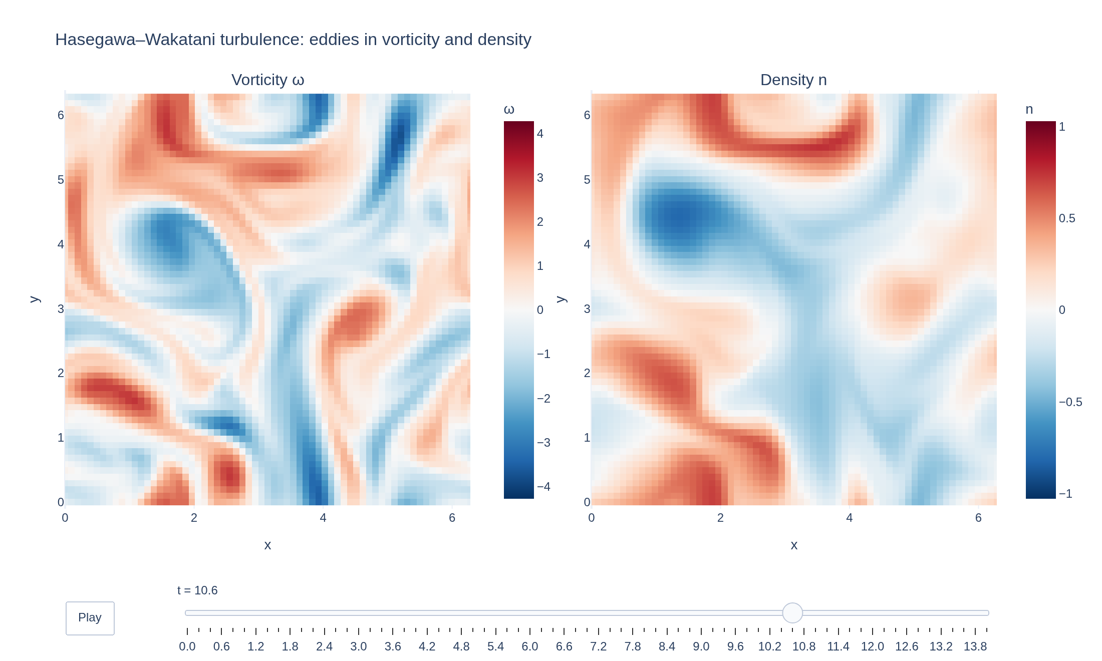
Hasegawa-Wakatani equations in 2D for drift-wave turbulence.

Overview

This is a reduced 2D drift-wave turbulence model. The electrostatic

potential is recovered from the vorticity at each step, and the coupled density-vorticity dynamics capture resistive drift-wave behavior without resolving full kinetic physics.

Use cases

This model is appropriate for:

2D resistive drift-wave turbulence studies
reduced electrostatic edge-plasma benchmarks
testing Poisson-coupled advection-diffusion solvers

Governing equations

PDEs solved by model:

Density equation:

\frac{\partial n}{\partial t} = C (ϕ - n) - [ϕ, n] - κ \partial_{y} ϕ + ν \nabla^{2 N} n

Vorticity equation:

\frac{\partial ω}{\partial t} = C (ϕ - n) - [ϕ, ω] + ν \nabla^{2 N} ω

Potential equation:

Δ ϕ = ω

where $[ϕ, n] = \partial_{x} ϕ \partial_{y} n - \partial_{y} ϕ \partial_{x} n$ , $C = C (x, y)$ and $κ$ and $ν$ are constants (at the moment only $N = 1$ is available).

Normalization

The electrostatic potential is scaled by the thermal-speed unit,

u^= v^_{th}, ϕ^= u^x^.

Discretization

Time integration is performed by the following propagators (in sequence):

Diagnostics

The following scalars are tracked during simulation:

No default scalar diagnostics are defined by this model.

Examples

Hasegawa–Wakatani drift-wave turbulence

Broadband fluctuations break into interacting density and vorticity eddies in a periodic plasma slab, while nonlinear E×B transport moves part of the kinetic energy into a banded zonal flow. The initial density and vorticity fluctuations use the same phases: $n(x,y,0)=0.12\sum_{\mathbf{k}}w_{\mathbf{k}}\cos(\mathbf{k}\cdot\mathbf{x}+\theta_{\mathbf{k}}),$ $\omega(x,y,0)=0.12\sum_{\mathbf{k}}|\mathbf{k}|^2w_{\mathbf{k}}\cos(\mathbf{k}\cdot\mathbf{x}+\theta_{\mathbf{k}}).$ Here $k_x,k_y\in\{1,\ldots,6\}$ , $2\le|\mathbf{k}|^2\le36$ and $\sum_{\mathbf{k}}w_{\mathbf{k}}^2=1$ ; random phases and weights use seed 1701.