HasegawaWakatani · Drift-wave turbulence
Hasegawa–Wakatani drift-wave turbulence
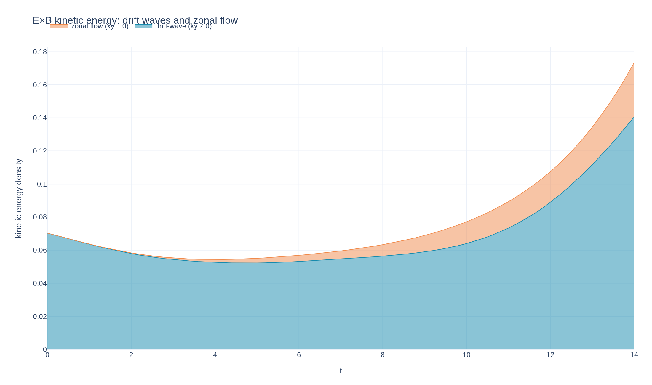
Broadband fluctuations break into interacting density and vorticity eddies in a periodic plasma slab, while nonlinear E×B transport moves part of the kinetic energy into a banded zonal flow.
Loading interactive figure…
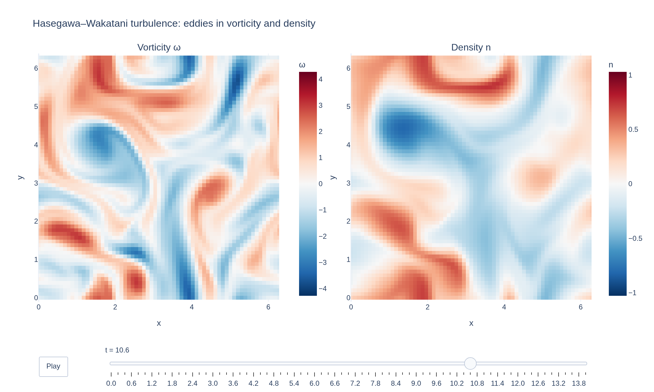
Loading interactive figure…
Physical problem
Eddies self-organizing into zonal flow
Broadband fluctuations break into interacting density and vorticity eddies in a periodic plasma slab, while nonlinear E×B transport moves part of the kinetic energy into a banded zonal flow.
PDEs solved by model:
Density equation:
Vorticity equation:
Potential equation:
where , and and are constants (at the moment only is available).
Simulation geometry
Domain used in this run
The actual Cuboid geometry reconstructed from this run's metadata. Switch between the 3D view and physical-coordinate slices.
Domain
Cuboid
Mapping
Loading Cuboid…
Parameters
| Parameter | Value | Description |
|---|---|---|
| Loading parameters… | ||
- Model
- HasegawaWakatani
- Grid
- 64 × 64 × 1
- FEEC degree
- 2 × 2 × 1
- Evolution
- 350 steps
- Visualization
- Plotly
Performance
Profiling
Struphy's built-in scope-profiler instruments every propagator, pusher and solver call — these are the real per-call timings from the run above.
Durations
Gantt (rank 0)
Region statistics
| Region | Count | Avg (s) | Min (s) | Max (s) | Total (s) |
|---|
Complete source
Simulation script
Requires Struphy with compiled kernels and Plotly. Run struphy compile once, then execute python hasegawa-wakatani.py.
"""Hasegawa-Wakatani drift-wave turbulence and the birth of zonal flow.

Broadband density and vorticity perturbations evolve on a doubly periodic
plane.  The background density gradient drives drift-wave structure while
nonlinear E×B advection transfers energy across scales and into the ky = 0
zonal flow.

The run is deliberately two-dimensional and saves only every fifth step, so
it remains a manageable gallery calculation while retaining the turbulent
eddies and the slow reorganization of their energy.

Requires Struphy 3.3 with compiled kernels (``struphy compile``).
"""

import numpy as np
import plotly.graph_objects as go

from struphy import DerhamOptions, EnvironmentOptions, Simulation, Time, domains, equils, grids
from struphy.initial.base import GenericPerturbation
from struphy.models import HasegawaWakatani
from struphy.ode.utils import ButcherTableau

# A square periodic slab.  The third direction is inactive, making this a
# genuinely 2D fluid calculation rather than a thin 3D one.
length = 2 * np.pi
model = HasegawaWakatani()
domain = domains.Cuboid(r1=length, r2=length)
equil = equils.HomogenSlab()
grid = grids.TensorProductGrid(num_elements=(64, 64, 1))
derham_opts = DerhamOptions(degree=(2, 2, 1))
time_opts = Time(dt=0.04, Tend=14.0, split_algo="LieTrotter")

# C couples density and potential, kappa supplies the background-gradient
# drive, and weak diffusion removes only the smallest resolved scales.  RK4
# is useful here because all three effects are advanced explicitly.
# The periodic Laplacian has an arbitrary constant mode. A small identity
# stabilization fixes that gauge and keeps the iterative solve inexpensive;
# it changes the k=1 response by less than one percent.
model.propagators.poisson.options = model.propagators.poisson.Options(stab_eps=0.01)
model.propagators.hw.options = model.propagators.hw.Options(
    coupling=1.0,
    kappa=1.0,
    nu=0.002,
    butcher=ButcherTableau(algo="rk4"),
)

# Use a reproducible, smooth broadband seed instead of grid-scale white
# noise.  Starting at finite amplitude avoids spending most of this compact
# gallery run waiting for the linear instability to leave the noise floor.
rng = np.random.default_rng(1701)
wave_numbers = np.array(
    [(kx, ky) for kx in range(1, 7) for ky in range(1, 7) if 2 <= kx**2 + ky**2 <= 36],
    dtype=int,
)
phases = rng.uniform(0.0, 2 * np.pi, len(wave_numbers))
weights = rng.normal(size=len(wave_numbers))
weights /= np.sqrt(np.sum(weights**2))


def broadband_field(x, y, z, *, laplacian=False):
    """A deterministic broadband potential, or its negative Laplacian."""
    result = np.zeros_like(x + y + z, dtype=float)
    for (kx, ky), phase, weight in zip(wave_numbers, phases, weights):
        factor = kx**2 + ky**2 if laplacian else 1.0
        result += factor * weight * np.cos(kx * x + ky * y + phase)
    return result


def initial_density(x, y, z):
    return 0.12 * broadband_field(x, y, z)


def initial_vorticity(x, y, z):
    # PoissonSolve uses the weak form -Delta(phi) = omega.
    return 0.12 * broadband_field(x, y, z, laplacian=True)


model.plasma.density.add_perturbation(GenericPerturbation(initial_density, given_in_basis="physical"))
model.plasma.vorticity.add_perturbation(GenericPerturbation(initial_vorticity, given_in_basis="physical"))

env = EnvironmentOptions(
    out_folders="struphy_gallery_runs",
    sim_folder="hasegawa_wakatani",
    save_step=5,
    save_restart=False,
)
sim = Simulation(
    model=model,
    name="Hasegawa–Wakatani drift-wave turbulence",
    description=(
        "Broadband fluctuations break into interacting density and vorticity "
        "eddies in a periodic plasma slab, while nonlinear E×B transport "
        "moves part of the kinetic energy into a banded zonal flow."
    ),
    env=env,
    time_opts=time_opts,
    domain=domain,
    equil=equil,
    grid=grid,
    derham_opts=derham_opts,
)


if __name__ == "__main__":
    from plotly.subplots import make_subplots

    from _gallery import export_profiling, merge_metadata, save_extra_figure, save_figure

    output = sim.run(profiling_activated=True)
    output.pproc(celldivide=1)

    density = output.evaluate("plasma/density").isel(e3=0, drop=True)
    vorticity = output.evaluate("plasma/vorticity").isel(e3=0, drop=True)
    potential = output.evaluate("em_fields/phi").isel(e3=0, drop=True)
    times = np.asarray(density.t)
    if times[-1] < time_opts.Tend - env.save_step * time_opts.dt:
        raise RuntimeError("Hasegawa-Wakatani simulation ended before the requested final time")

    # xarray stores these fields as (t, e1, e2); Plotly heatmaps expect
    # (row=y, column=x), hence the final transpose in each frame.
    x = np.asarray(density.e1) * length
    y = np.asarray(density.e2) * length
    n_values = density.transpose("t", "e1", "e2").values
    w_values = vorticity.transpose("t", "e1", "e2").values
    if not (np.isfinite(n_values).all() and np.isfinite(w_values).all()):
        raise RuntimeError("Non-finite Hasegawa-Wakatani field: refusing to publish the run")

    # Fixed, symmetric colour limits make changes between frames meaningful;
    # a high percentile keeps an isolated extremum from washing out the eddies.
    n_limit = float(np.percentile(np.abs(n_values), 99.7))
    w_limit = float(np.percentile(np.abs(w_values), 99.7))
    picks = np.unique(np.linspace(0, len(times) - 1, min(120, len(times)), dtype=int))

    def field_traces(index, *, colorbars=False):
        return [
            go.Heatmap(
                z=w_values[index].T,
                x=x,
                y=y,
                zmin=-w_limit,
                zmax=w_limit,
                colorscale="RdBu_r",
                colorbar={"title": "ω", "x": 0.46} if colorbars else None,
                showscale=colorbars,
            ),
            go.Heatmap(
                z=n_values[index].T,
                x=x,
                y=y,
                zmin=-n_limit,
                zmax=n_limit,
                colorscale="RdBu_r",
                colorbar={"title": "n"} if colorbars else None,
                showscale=colorbars,
            ),
        ]

    figure = make_subplots(rows=1, cols=2, horizontal_spacing=0.13, subplot_titles=("Vorticity ω", "Density n"))
    still_position = len(picks) * 3 // 4
    still_index = picks[still_position]
    figure.add_trace(field_traces(still_index, colorbars=True)[0], row=1, col=1)
    figure.add_trace(field_traces(still_index, colorbars=True)[1], row=1, col=2)
    figure.frames = [
        go.Frame(name=f"{times[index]:.1f}", data=field_traces(index), traces=[0, 1])
        for index in picks
    ]
    figure.update_layout(
        title="Hasegawa–Wakatani turbulence: eddies in vorticity and density",
        template="plotly_white",
        margin={"l": 65, "r": 50, "t": 90, "b": 135},
        updatemenus=[{
            "type": "buttons", "showactive": False, "x": 0.0, "xanchor": "left", "y": -0.22,
            "buttons": [{"label": "Play", "method": "animate", "args": [None, {"frame": {"duration": 45, "redraw": True}, "transition": {"duration": 0}, "fromcurrent": True}]}],
        }],
        sliders=[{
            "active": still_position, "x": 0.12, "len": 0.88, "y": -0.12, "currentvalue": {"prefix": "t = "},
            "steps": [{"args": [[frame.name], {"frame": {"duration": 0, "redraw": True}, "mode": "immediate"}], "label": frame.name, "method": "animate"} for frame in figure.frames],
        }],
    )
    for column in (1, 2):
        figure.update_xaxes(title_text="x", range=[0, length], constrain="domain", row=1, col=column)
        figure.update_yaxes(title_text="y", range=[0, length], scaleanchor="x" if column == 1 else "x2", scaleratio=1, row=1, col=column)
    save_figure(figure, "hasegawa-wakatani", width=1100, height=660)

    # E×B kinetic energy is |grad(phi)|²/2.  Averaging phi over y selects
    # ky = 0; its remaining y-directed velocity is the zonal flow.  Spectral
    # derivatives respect the doubly periodic domain and make the split exact
    # up to roundoff on the sampled grid.
    # The sampled periodic grid includes the repeated right/top boundary.
    # Remove it before the FFT so it is not counted as a second grid point.
    phi = potential.transpose("t", "e1", "e2").values[:, :-1, :-1]
    nx, ny = phi.shape[1:]
    kx = 2 * np.pi * np.fft.fftfreq(nx, d=length / nx)[:, None]
    ky = 2 * np.pi * np.fft.fftfreq(ny, d=length / ny)[None, :]
    phi_hat = np.fft.fft2(phi, axes=(1, 2))
    velocity_x = np.fft.ifft2(-1j * ky * phi_hat, axes=(1, 2)).real
    velocity_y = np.fft.ifft2(1j * kx * phi_hat, axes=(1, 2)).real
    total_energy = 0.5 * np.mean(velocity_x**2 + velocity_y**2, axis=(1, 2))
    zonal_velocity = np.mean(velocity_y, axis=2)
    zonal_energy = 0.5 * np.mean(zonal_velocity**2, axis=1)
    drift_wave_energy = np.maximum(total_energy - zonal_energy, 0.0)

    energy_figure = go.Figure()
    energy_figure.add_scatter(x=times, y=drift_wave_energy, mode="lines", name="drift-wave (ky ≠ 0)", stackgroup="energy", line={"color": "#168aad", "width": 1})
    energy_figure.add_scatter(x=times, y=zonal_energy, mode="lines", name="zonal flow (ky = 0)", stackgroup="energy", line={"color": "#f08a4b", "width": 1})
    energy_figure.update_layout(
        title="E×B kinetic energy: drift waves and zonal flow",
        xaxis_title="t",
        yaxis_title="kinetic energy density",
        template="plotly_white",
        margin={"l": 80, "r": 30, "t": 80, "b": 60},
        legend={"orientation": "h", "y": 1.1},
    )
    figures = [save_extra_figure(
        energy_figure,
        "hasegawa-wakatani",
        "zonal-energy",
        alt="Stacked kinetic energy in drift-wave and zonal-flow modes",
        caption=(
            "The E×B kinetic energy split by poloidal Fourier mode. The ky = 0 part is the banded "
            "zonal flow; everything with ky ≠ 0 is assigned to the turbulent drift-wave field."
        ),
    )]

    final_zonal_fraction = float(zonal_energy[-1] / total_energy[-1]) if total_energy[-1] else 0.0
    merge_metadata(
        "hasegawa-wakatani",
        finalZonalEnergyFraction=final_zonal_fraction,
        peakZonalEnergyFraction=float(np.max(zonal_energy / np.maximum(total_energy, np.finfo(float).tiny))),
        figures=figures,
        **export_profiling(sim, "hasegawa-wakatani"),
    )
See the post-processing guide for more ways to inspect the result.