2 - Parameter/launch files

We have seen in Tutorial 1 how to launch a Struphy simulation from scratch. In addition, for each model there exist pre-defined “launch files” that can be used as templates to set up more complicated simulations.

Launch files are Python scripts (.py) that can be executed with the Python interpreter. For each model (PDE), the default launch file can be generated from the console. For example, a launch file of the model Vlasov can be generated from

struphy params Vlasov

This will create a file params_Vlasov.py in the current working directory. To see its contents, open the file in your preferred editor or type

cat params_Vlasov.py

To run the model type

python params_Vlasov.py

One can modify the launch file to set parameters for a specific simulation.

We shall discuss this launch file in what follows. Launch files of all models have a similar structure.

Part 1: Description of the simulation

This part contains a string describing the contents of the simulation. A short summary of 3-4 sentences should usually be enough. We advise you to write this description for your simulations, as it will help to track and retrieve past simulations.

description = """
This is the default simulation for the model Vlasov.
It is meant to be a template for users to set up their own simulations with this model.
It contains all the necessary components of a Struphy simulation, including the model,
the environment options, the time stepping options, the geometry, the equilibrium,
the grid, the Derham options, and the initial conditions.
Users can modify this file to set up their own simulations with different parameters and initial conditions.
"""

print("\nRunning Vlasov.")
print(description)

Running Vlasov.

This is the default simulation for the model Vlasov.
It is meant to be a template for users to set up their own simulations with this model.
It contains all the necessary components of a Struphy simulation, including the model,
the environment options, the time stepping options, the geometry, the equilibrium,
the grid, the Derham options, and the initial conditions.
Users can modify this file to set up their own simulations with different parameters and initial conditions.

Part 2: Import Struphy API

In this part we import several modules and classes from the Struphy API. The API contains the user-facing components of Struphy and can be used to set up the launch file.

from struphy import (
    BaseUnits,
    DerhamOptions,
    EnvironmentOptions,
    FieldsBackground,
    Simulation,
    Time,
    domains,
    equils,
    grids,
    perturbations,
)

# For particles:
from struphy import (
    BinningPlot,
    BoundaryParameters,
    KernelDensityPlot,
    LoadingParameters,
    WeightsParameters,
    maxwellians,
)

All parameter files import the first set of modules and classes above; the second set is imported only when particles are part of the discrete model.

Part 3: Instance of the model

Here, a light-weight instance of the model is created, without allocating memory. The light-weight instance is used to set some model-specific parameters for each species, and to maybe exclude some propagators in some models.

In the light-weight instance, we can

1. set species properties like charge- and mass number

2. exclude variables from saving

3. set particle initial conditions (see below)

4. set Propagator options (see below)

from struphy.models import Vlasov

# Units
base_units = BaseUnits()

# Model instance
model = Vlasov(base_units=base_units)

# List all variables and decide whether to save their data
model.kinetic_ions.var.save_data = True

Part 4: Instance of the simulation

At the heart of Struphy is the Simulation class which was already introduced in Tutorial 1. In this part of the launch file we create an instance of this class, which takes the following types as input arguments:

• EnvironmentOptions

• BaseUnits

• Time

• Domain

• FluidEquilibrium

• Grid

• DerhamOptions

Check the respective classes for available arguments.

# Environment options
env = EnvironmentOptions()

# Time stepping
time_opts = Time(dt=0.2, Tend=10.0)

# Geometry
l1 = -5.0
r1 = 5.0
l2 = -7.0
r2 = 7.0
l3 = -1.0
r3 = 1.0
domain = domains.Cuboid(l1=l1, r1=r1, l2=l2, r2=r2, l3=l3, r3=r3)

# Fluid equilibrium (can be used as part of initial conditions)
equil = None

# Grid
grid = grids.TensorProductGrid()

# Derham options
derham_opts = DerhamOptions()

Once we have defined the input arguments, we can create our simulation object:

# Simulation object
sim = Simulation(
    model=model,
    params_path=None,
    env=env,
    time_opts=time_opts,
    domain=domain,
    equil=equil,
    grid=grid,
    derham_opts=derham_opts,
)

Part 5: Particle parameters

In case of a particle model, in this part one can set parameters regarding marker drawing, boundary conditions, weight computation, box sorting and data saving:

loading_params = LoadingParameters(Np=15)
weights_params = WeightsParameters()
boundary_params = BoundaryParameters(bc=("reflect", "reflect", "periodic"))
model.kinetic_ions.set_markers(
    loading_params=loading_params, weights_params=weights_params, boundary_params=boundary_params
)

model.kinetic_ions.set_sorting_boxes()
model.kinetic_ions.set_save_data(n_markers=1.0)

Part 6: Propagator options

A model is a collection of “propagators” which perform the time stepping. Each propagator refers to part of a single time step and can be viewed as a splitting step. For instance, if only a single propagator is present in a model, then all variables of the model are updated by this propagator. If two or more propagators are present, they are executed in sequence, according to the chosen splitting algorithm (Lie-Trotter, Strang, etc.).

For each propagator, the options can be set in this part:

# propagator options
model.propagators.push_vxb.options = model.propagators.push_vxb.Options()
model.propagators.push_eta.options = model.propagators.push_eta.Options()

Part 7: Initial conditions

Initial conditions for the variables of a model are the sum of background(s) and perturbation(s). If backgrounds or perturbations are not specified, they are assumed to be zero. Other important points:

• For kinetic species the background is mandatory.

• For kinetic species, if add_initial_condition() is not called, the background is taken as the kinetic initial condition.

• For kinetic species the perturbations are added to the moments of the distribution function (defined as tuples).

# initial conditions (background + perturbation)
perturbation = None

background = maxwellians.Maxwellian3D(n=(1.0, perturbation))
model.kinetic_ions.var.add_background(background)

Part 8: run()

In the final part of the launch file, the method Simulation.run() is called, but only when the file is launched from the console (not when it is imported). The run command will allocate memory and run the specified simulation. The verbose flag controls the screen output during the simulation.

sim.run(verbose=False)

Starting simulation run for model Vlasov ...
Struphy run finished.

Post processing: the pproc method

Aside from run, the Simulation class has the method pproc for post-processing raw simulation data:

sim.pproc()

100%|██████████| 51/51 [00:00<00:00, 640.88it/s]

In case we do not have the simulation object, but only the stored data, we can call the PostProcessor class. This class is called internally by (pproc()):

from struphy import PostProcessor
import os

path = os.path.join(os.getcwd(), "sim_1")

pp = PostProcessor(path_out=path)
pp.process()

100%|██████████| 51/51 [00:00<00:00, 859.05it/s]

Plotting: the load_plotting_data method

After post-processing, the generated data can be loaded via Simulation.load_plotting_data().

sim.load_plotting_data()

In case we do not have the simulation object, but only the stored data, we can call the PlottingData class. This class is called internally by (load_plotting_data()):

from struphy import PlottingData

pdata = PlottingData(path_out=path)
pdata.load()

Plotting particle orbits

Let’s inspect the orbits of the simulation:

print(sim.orbits)

    kinetic_ions, shape = (51, 15, 8)
        Number of time points: 51
        Number of particles:   15
        Number of attributes:  8

orbits = sim.orbits.kinetic_ions
print(f"{orbits.shape = }")
Nt = sim.orbits.kinetic_ions.shape[0]
Np = sim.orbits.kinetic_ions.shape[1]

orbits.shape = (51, 15, 8)

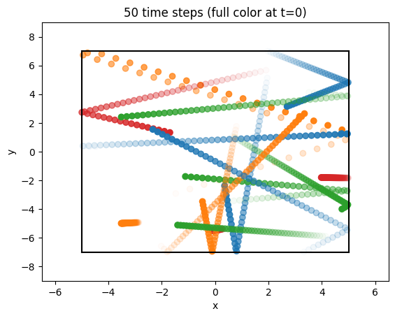
Let us plot the orbits:

import numpy as np
from matplotlib import pyplot as plt

fig = plt.figure()
ax = fig.gca()

colors = ["tab:blue", "tab:orange", "tab:green", "tab:red"]

# create alpha for color scaling
Tend = time_opts.Tend
alpha = np.linspace(1.0, 0.0, Nt + 1)

# loop through particles, plot all time steps
for i in range(Np):
    ax.scatter(orbits[:, i, 0], orbits[:, i, 1], c=colors[i % 4], alpha=alpha)

ax.plot([l1, l1], [l2, r2], "k")
ax.plot([r1, r1], [l2, r2], "k")
ax.plot([l1, r1], [l2, l2], "k")
ax.plot([l1, r1], [r2, r2], "k")
ax.set_xlabel("x")
ax.set_ylabel("y")
ax.set_xlim(-6.5, 6.5)
ax.set_ylim(-9, 9)
ax.set_title(f"{int(Nt - 1)} time steps (full color at t=0)");