1 - Struphy simulations

In this tutorial we will create a basic simulation with Struphy, run it, do post-processing and plot the data.

The first step is to choose a model (that is the PDE) we want to solve:

from struphy import models

model = models.Maxwell()

We can print the info of the model to see the governing equations and the physical meaning of the variables:

model.info()

Maxwell's equations in vacuum for electromagnetic field evolution.

To see detailed information on the model, run the following methods:

Maxwell.pde()
Maxwell.normalization()
Maxwell.scalar_quantities()
Maxwell.discretization()
Maxwell.long_description()
Maxwell.examples()
Maxwell.use_cases()
Maxwell.cannot_be_used_for()

We now feed the light-weight model instance into a simulation:

from struphy import Simulation

sim = Simulation(model=model)

Depending on the model, there are many parameters that can be set for a simulation. You can inspect the Simulation class for how to do this. Setting initial conditions for the model’s variables will be discussed below.

It is straightforward to run a simulation:

sim.run()

Starting simulation run for model Maxwell ...
Struphy run finished.

The screen output shows several things:

1. The default options for the propagator ‘Maxwell’, which is the only propagator in this model.

2. The initial conditions (background + perturbation) for the two variables of the model, both initialized as zero here.

3. Some information about the stages of the run.

It is possible to re-run the simulation, but be careful: existing data will be deleted! We shall re-run the same simulation with more verbose output:

sim.run(verbose=True)

Starting simulation run for model Maxwell ...
Struphy run finished.

In verbose mode, we see some more information on the individual time steps during the simulation. Moreover, some info on the allocation and assembly of simulation objects are printed.

Our next aim is to set an initial condition for the electric field. To find out the species and variables of a model, all we need to do is print the model object:

print(model)

Maxwell
    em_fields:
        e_field:    FEECVariable (Hcurl)
        b_field:    FEECVariable (Hdiv)

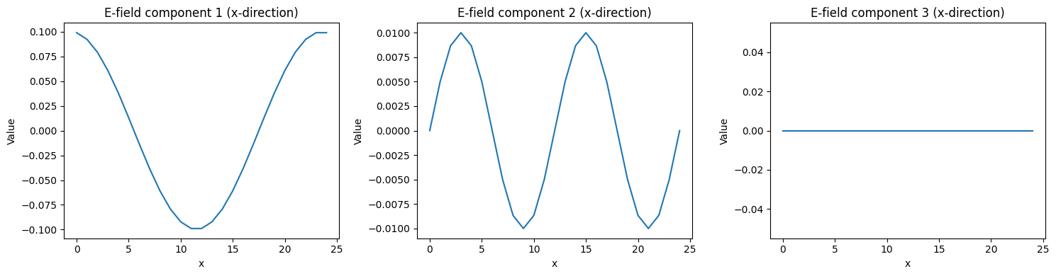
We want a cosine function for the first component and a sine function for the second component, both in x-direction, of the electric field. Pre-defined functions can be loaded from the module perturbations:

from struphy import perturbations

fun1 = perturbations.ModesCos(ls=(1,), amps=(1e-1,), comp=0)
fun2 = perturbations.ModesSin(ls=(2,), amps=(1e-2,), comp=1)

model.em_fields.e_field.add_perturbation(perturbation=fun1)
model.em_fields.e_field.add_perturbation(perturbation=fun2)

We can check the perturbations of a given variable (try to add another perturbation and check again):

model.em_fields.e_field.show_perturbations()

Let us now run the simulation with the changed initial condition:

sim.run()

Starting simulation run for model Maxwell ...
Struphy run finished.

We can immediately post-process the simulation with default settings:

sim.pproc()

100%|██████████| 2/2 [00:00<00:00, 301.42it/s]
100%|██████████| 4/4 [00:00<00:00, 12.88it/s]
100%|██████████| 4/4 [00:00<00:00, 935.29it/s]

After post-processing, the plotting data can be loaded:

sim.load_plotting_data()

Let us plot the initial condition of the electric field. For this we have to inspect the spline_values of the simulation:

sim.spline_values

<struphy.post_processing.post_processing_tools.SplineValues at 0x7f1dbfed3e80>

In this example there is just one species em_fields holding the two variables b_field_log and e_field_log. The data can be inspected as follows:

e_field = sim.spline_values.em_fields.e_field_log
print(e_field)

type(self.data) = <class 'dict'>
len(self.data) = 4
key = np.float64(0.0)    shape = [(25, 11, 2), (25, 11, 2), (25, 11, 2)]
key = np.float64(0.01)   shape = [(25, 11, 2), (25, 11, 2), (25, 11, 2)]
key = np.float64(0.02)   shape = [(25, 11, 2), (25, 11, 2), (25, 11, 2)]
key = np.float64(0.03)   shape = [(25, 11, 2), (25, 11, 2), (25, 11, 2)]

The data is thus a dictionary where the keys are simulation times in normalized units, for every time step. The actual spline values are the corresponding values in the form of lists holding numpy arrays with the indicated shape. The shape matches the grid size seen in the above output.

Let us plot the initial condition in x-direction of the electric field:

e_init = e_field.data[0.0]
print(f"{e_init[1].shape = }")

from matplotlib import pyplot as plt

fig, axes = plt.subplots(1, 3, figsize=(15, 4))

# Plot 1: First component in x-direction
axes[0].plot(e_init[0][:, 0, 0])
axes[0].set_title("E-field component 1 (x-direction)")
axes[0].set_xlabel("x")
axes[0].set_ylabel("Value")

# Plot 2: Add your second plot
axes[1].plot(e_init[1][:, 0, 0])
axes[1].set_title("E-field component 2 (x-direction)")
axes[1].set_xlabel("x")
axes[1].set_ylabel("Value")

# Plot 3: Add your third plot
axes[2].plot(e_init[2][:, 0, 0])
axes[2].set_title("E-field component 3 (x-direction)")
axes[2].set_xlabel("x")
axes[2].set_ylabel("Value")

plt.tight_layout()

e_init[1].shape = (25, 11, 2)