4 - Smoothed-particle hydrodynamics

Struphy provides several models for smoothed-particle hydrodynamics (SPH). In this tutorial, we shall explore

1. Pressure-less fluid flow in a Beltrami force field (model PressureLessSPH)

2. Gas expansion with SPH (model ViscousEulerSPH)

The parameter files discussed below can be obtained with the console commands

struphy params PressureLessSPH
struphy params ViscousEulerSPH

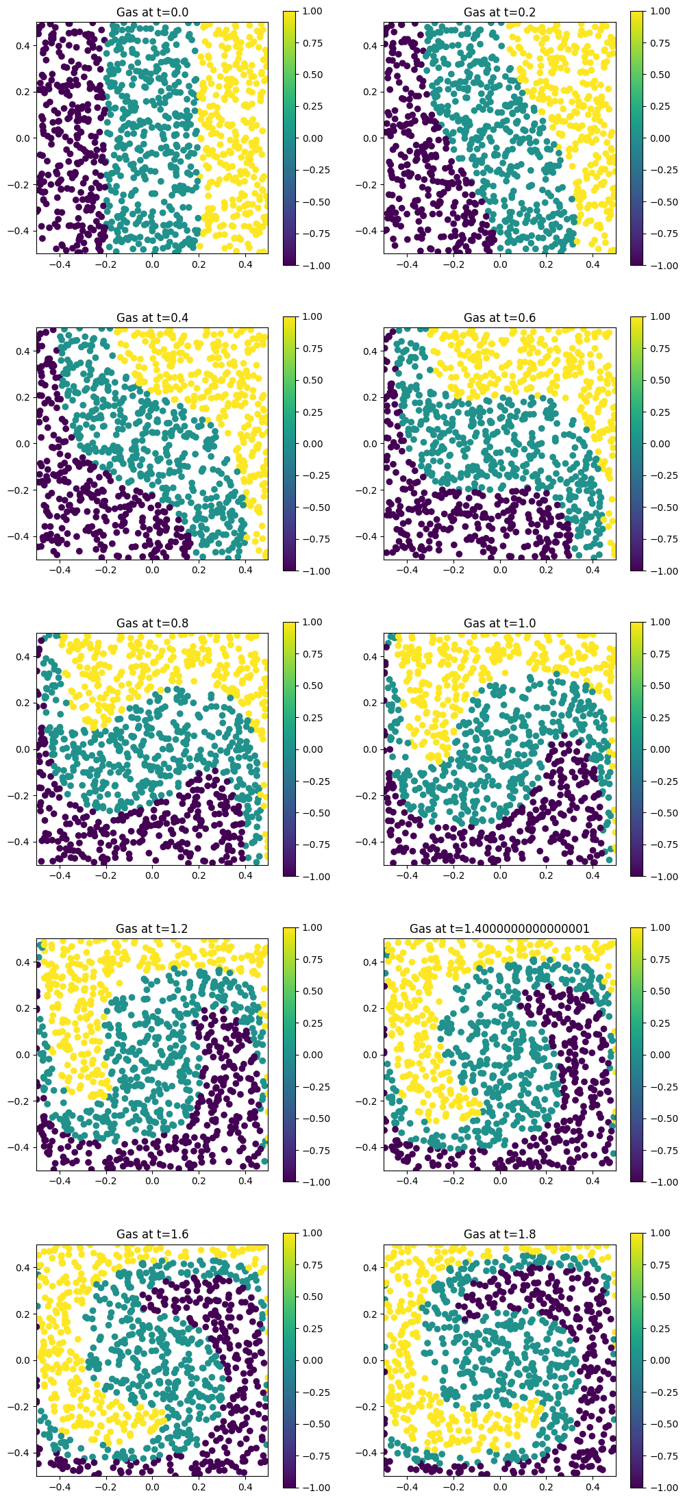
Pressure-less fluid flow in Beltrami force field

Let \(\mathbf u_0(\mathbf x)\) stand for an initial flow velocity field. Moreover, let \(\Omega \subset \mathbb R^3\) be a box (cuboid). We search for trajectories \((\mathbf x_p, \mathbf v_p): [0,T] \to \Omega \times \mathbb R^3\), \(p = 0, \ldots, N-1\) that satisfy

\[\begin{split}\begin{aligned} \dot{\mathbf x}_p &= \mathbf v_p\,,\qquad && \mathbf x_p(0) = \mathbf x_{p0}\,, \\[2mm] \dot{\mathbf v}_p &= -\nabla p(\mathbf x_p) \qquad && \mathbf v_p(0) = \mathbf u_0(\mathbf x_p(0))\,, \end{aligned}\end{split}\]

where \(p \in H^1(\Omega)\) is some given function. In what follows we shall set \(p\) to give a Beltrami force field to guide the fluid particles.

We start with the API imports:

from struphy import EnvironmentOptions, Time
from struphy import domains
from struphy import equils
from struphy import grids
from struphy import DerhamOptions
from struphy import (
    BinningPlot,
    BoundaryParameters,
    KernelDensityPlot,
    LoadingParameters,
    WeightsParameters,
)
from struphy import Simulation

We shall use the Strang splitting algorithm for the propagators, and simulate in Cartesian geometry (Cuboid):

# environment options
env = EnvironmentOptions()

# time stepping
time_opts = Time(dt=0.02, Tend=4, split_algo="Strang")

# geometry
l1 = -0.5
r1 = 0.5
l2 = -0.5
r2 = 0.5
l3 = 0.0
r3 = 1.0
domain = domains.Cuboid(l1=l1, r1=r1, l2=l2, r2=r2, l3=l3, r3=r3)

The Beltrami flow can be specified as a lambda function and then passed to GenericCartesianFluidEquilibrium. This fluid equilibrium will be set as initial condition below.

# construct Beltrami flow
import numpy as np


def u_fun(x, y, z):
    ux = -np.cos(np.pi * x) * np.sin(np.pi * y)
    uy = np.sin(np.pi * x) * np.cos(np.pi * y)
    uz = 0 * x
    return ux, uy, uz


p_fun = lambda x, y, z: 0.5 * (np.sin(np.pi * x) ** 2 + np.sin(np.pi * y) ** 2)
n_fun = lambda x, y, z: 1.0 + 0 * x

# put the functions in a generic equilibrium container
bel_flow = equils.GenericCartesianFluidEquilibrium(u_xyz=u_fun, p_xyz=p_fun, n_xyz=n_fun)

We will also need a grid and Derham complex for projecting the fluid equilibrium onto a spline basis:

# fluid equilibrium (can be used as part of initial conditions)
equil = None

# grid
grid = grids.TensorProductGrid(num_elements=(64, 64, 1))

# derham options
bcs = (("free", "free"), ("free", "free"), None)
derham_opts = DerhamOptions(degree=(3, 3, 1), bcs=bcs)

Let us now create the instance of the simulation:

# import model
from struphy.models import PressureLessSPH

# light-weight model instance
model = PressureLessSPH(epsilon=1.0)

sim = Simulation(model,
                 env=env,
                 time_opts=time_opts,
                 domain=domain,
                 equil=equil,
                 grid=grid,
                 derham_opts=derham_opts,)

/opt/hostedtoolcache/Python/3.10.20/x64/lib/python3.10/site-packages/struphy/models/species.py:195: UserWarning: Override equation parameter self.epsilon =1.0
  warnings.warn(f"Override equation parameter {self.epsilon =}")

In the next step, the light-weight instance of the model is created. We set the parameter epsilon to 1.0, appearing in the propagator PushVinEfield. Moreover, we launch with 1000 particles and save 100 % percent of them through n_markers=1.0.

loading_params = LoadingParameters(Np=1000)
weights_params = WeightsParameters()
boundary_params = BoundaryParameters(bc=("reflect", "reflect", "periodic"))
model.cold_fluid.set_markers(
    loading_params=loading_params,
    weights_params=weights_params,
    boundary_params=boundary_params,
)
model.cold_fluid.set_sorting_boxes(boxes_per_dim=(1, 1, 1))
model.cold_fluid.set_save_data(n_markers=1.0)

We now set the propagator options. Here, it is important to pass the pressure from the Beltrami flow as auxiliary field to push_v:

# propagator options
from struphy import ButcherTableau

butcher = ButcherTableau(algo="forward_euler")
model.propagators.push_eta.options = model.propagators.push_eta.Options(butcher=butcher)

phi = bel_flow.p0
model.propagators.push_v.options = model.propagators.push_v.Options(phi=phi)

The initial condition of the species is defined by a background function, plus possible perturbations, which we ignore here. The background of the species is set to the Beltrami flow:

# background, perturbations and initial conditions
model.cold_fluid.var.add_background(bel_flow)

Let us start the run, post-process the raw data, load the post-processed data and plot the particle trajectories:

sim.run()

Starting simulation run for model PressureLessSPH ...
Struphy run finished.

sim.pproc()

100%|██████████| 201/201 [00:01<00:00, 116.79it/s]

sim.load_plotting_data()

from matplotlib import pyplot as plt

plt.figure(figsize=(12, 28))

orbits = sim.orbits.cold_fluid

coloring = np.select(
    [orbits[0, :, 0] <= -0.2, np.abs(orbits[0, :, 0]) < +0.2, orbits[0, :, 0] >= 0.2], [-1.0, 0.0, +1.0]
)

dt = time_opts.dt
Nt = sim.t_grid.size - 1
interval = Nt / 20
plot_ct = 0
for i in range(Nt):
    if i % interval == 0:
        print(f"{i=}")
        plot_ct += 1
        plt.subplot(5, 2, plot_ct)
        ax = plt.gca()
        plt.scatter(orbits[i, :, 0], orbits[i, :, 1], c=coloring)
        plt.axis("square")
        plt.title("n0_scatter")
        plt.xlim(l1, r1)
        plt.ylim(l2, r2)
        plt.colorbar()
        plt.title(f"Gas at t={i * dt}")
    if plot_ct == 10:
        break

i=0
i=10
i=20
i=30
i=40
i=50
i=60
i=70
i=80
i=90

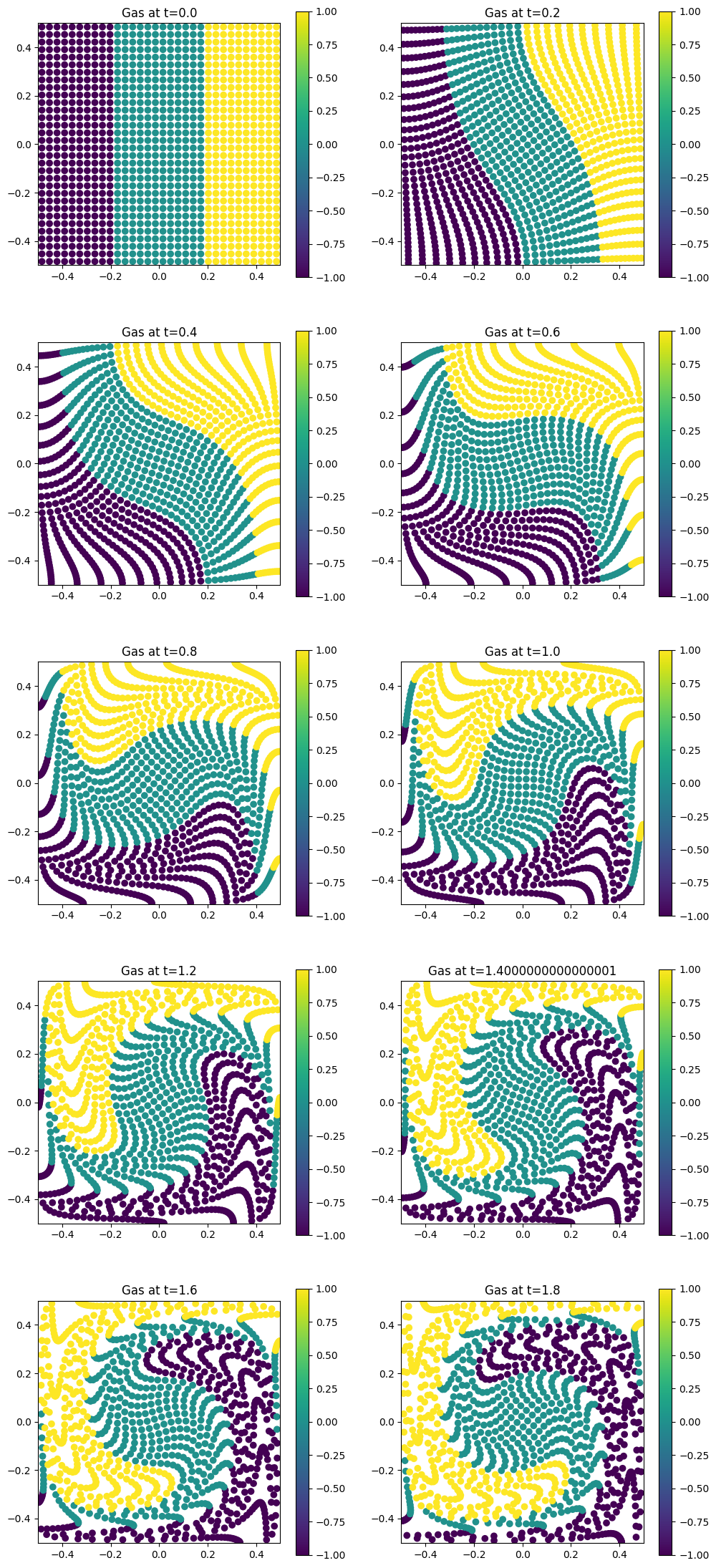
Let us perform another simulation, similar to the previous one. We will save the results in the folder sim_2:

# light-weight model instance
model = PressureLessSPH(epsilon=1.0)

# environment options
env = EnvironmentOptions(sim_folder="sim_2")

# simulation instance
sim_tess = sim.spawn_sister(model=model, env=env)

This time, we shall draw the markers on a regular grid obtained from a tesselation of the domain:

loading_params = LoadingParameters(ppb=4, loading="tesselation")
weights_params = WeightsParameters()
boundary_params = BoundaryParameters(bc=("reflect", "reflect", "periodic"))
model.cold_fluid.set_markers(
    loading_params=loading_params, weights_params=weights_params, boundary_params=boundary_params, bufsize=0.5
)
model.cold_fluid.set_sorting_boxes(boxes_per_dim=(16, 16, 1))
model.cold_fluid.set_save_data(n_markers=1.0)

# propagator options
from struphy import ButcherTableau

butcher = ButcherTableau(algo="forward_euler")
model.propagators.push_eta.options = model.propagators.push_eta.Options(butcher=butcher)

phi = bel_flow.p0
model.propagators.push_v.options = model.propagators.push_v.Options(phi=phi)

# background, perturbations and initial conditions
model.cold_fluid.var.add_background(bel_flow)

sim_tess.run()

Starting simulation run for model PressureLessSPH ...
Struphy run finished.

sim_tess.pproc()

100%|██████████| 201/201 [00:01<00:00, 122.55it/s]

sim_tess.load_plotting_data()

from matplotlib import pyplot as plt

plt.figure(figsize=(12, 28))

orbits = sim_tess.orbits.cold_fluid

coloring = np.select(
    [orbits[0, :, 0] <= -0.2, np.abs(orbits[0, :, 0]) < +0.2, orbits[0, :, 0] >= 0.2], [-1.0, 0.0, +1.0]
)

dt = time_opts.dt
Nt = sim_tess.t_grid.size - 1
interval = Nt / 20
plot_ct = 0
for i in range(Nt):
    if i % interval == 0:
        print(f"{i=}")
        plot_ct += 1
        plt.subplot(5, 2, plot_ct)
        ax = plt.gca()
        plt.scatter(orbits[i, :, 0], orbits[i, :, 1], c=coloring)
        plt.axis("square")
        plt.title("n0_scatter")
        plt.xlim(l1, r1)
        plt.ylim(l2, r2)
        plt.colorbar()
        plt.title(f"Gas at t={i * dt}")
    if plot_ct == 10:
        break

i=0
i=10
i=20
i=30
i=40
i=50
i=60
i=70
i=80
i=90

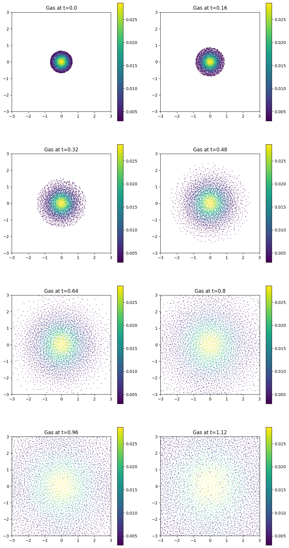
Gas expansion

We use SPH to solve Euler’s equations (model ViscousEulerSPH):

\[\begin{split}\begin{aligned} \partial_t \rho + \nabla \cdot (\rho \mathbf u) &= 0\,, \\[2mm] \rho(\partial_t \mathbf u + \mathbf u \cdot \nabla \mathbf u) &= - \nabla \left(\rho^2 \frac{\partial \mathcal U(\rho, S)}{\partial \rho} \right)\,, \\[2mm] \partial_t S + \mathbf u \cdot \nabla S &= 0\,, \end{aligned}\end{split}\]

where \(S\) denotes the entropy per unit mass and the internal energy per unit mass is

\[\mathcal U(\rho, S) = \kappa(S) \log \rho\,.\]

The SPH discretization leads to ODEs for \(N\) particles indexed by \(p\),

\[\begin{split}\begin{aligned} \dot{\mathbf x}_p &= \mathbf v_p\,,\qquad && \mathbf x_p(0) = \mathbf x_{p0}\,, \\[2mm] \dot{\mathbf v}_p &= -\kappa_{p}(0) \sum_{i=1}^N w_i \left(\frac{1}{\rho^{N,h}(\mathbf x_p)} + \frac{1}{\rho^{N,h}(\mathbf x_i)} \right) \nabla W_h(\mathbf x_p - \mathbf x_i) \qquad && \mathbf v_p(0) = \mathbf u(\mathbf x_p(0))\,, \end{aligned}\end{split}\]

where the smoothed density reads

\[\rho^{N,h}(\mathbf x) = \sum_{j=1}^N w_j W_h(\mathbf x - \mathbf x_j)\,,\]

with weights \(w_p = const.\) and where \(W_h(\mathbf x)\) is a suitable smoothing kernel. The velocity update is performed with the Propagator PushVinSPHpressure.

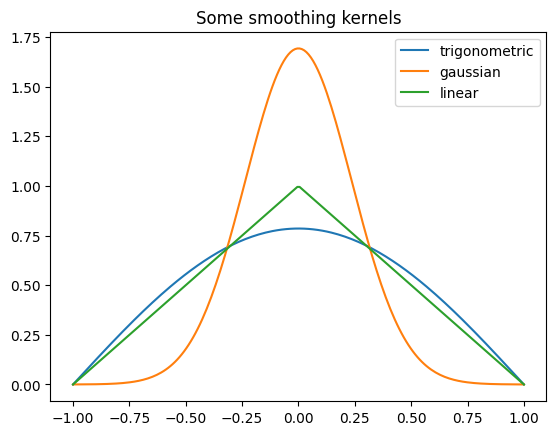
We shall now compute a gas expansion in 2d (nonlinear example). First, check out some of the smoothing kernels available for SPH evaluations:

from struphy.pic.sph_smoothing_kernels import gaussian_uni, linear_uni, trigonometric_uni

x = np.linspace(-1, 1, 200)
out1 = np.zeros_like(x)
out2 = np.zeros_like(x)
out3 = np.zeros_like(x)

for i, xi in enumerate(x):
    out1[i] = trigonometric_uni(xi, 1.0)
    out2[i] = gaussian_uni(xi, 1.0)
    out3[i] = linear_uni(xi, 1.0)
plt.plot(x, out1, label="trigonometric")
plt.plot(x, out2, label="gaussian")
plt.plot(x, out3, label="linear")
plt.title("Some smoothing kernels")
plt.legend()

<matplotlib.legend.Legend at 0x7f99b7943670>

We start with the generic imports and also import the model ViscousEulerSPH:

from struphy import DerhamOptions, EnvironmentOptions, Time
from struphy import domains
from struphy import grids
from struphy import (
    BoundaryParameters,
    LoadingParameters,
    WeightsParameters,
)
from struphy import Simulation

# import model
from struphy.models import ViscousEulerSPH

Here, it is important to set the base unit kBT in order to derive the velocity unit:

# environment options
env = EnvironmentOptions()

# time stepping
time_opts = Time(dt=0.04, Tend=1.6, split_algo="Strang")

# geometry
l1 = -3.0
r1 = 3.0
l2 = -3.0
r2 = 3.0
l3 = 0.0
r3 = 1.0
domain = domains.Cuboid(l1=l1, r1=r1, l2=l2, r2=r2, l3=l3, r3=r3)

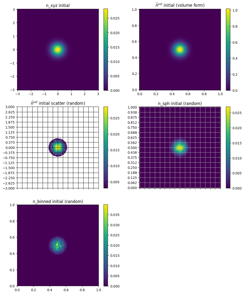
As background, which goes into the initial condition below, we define a Gaussian blob in the xy-plane:

# gaussian initial blob
import numpy as np

T_h = 0.2
gamma = 5 / 3
n_fun = lambda x, y, z: np.exp(-(x**2 + y**2) / T_h) / 35

blob = equils.GenericCartesianFluidEquilibrium(n_xyz=n_fun)

We also need a grid and Derham complex for projecting the fluid background on a spline basis:

# fluid equilibrium (can be used as part of initial conditions)
equil = None

# grid
grid = grids.TensorProductGrid(num_elements=(64, 64, 1))

# derham options
bcs = (("free", "free"), ("free", "free"), None)
derham_opts = DerhamOptions(degree=(3, 3, 1), bcs=bcs)

Now we create the light-weight instance of ViscousEulerSPH, without the optional propagator for particles in a magnetic background field, and instantiate the simulation:

# light-weight model instance
model = ViscousEulerSPH(with_B0=False, with_viscosity=False)

sim = Simulation(model,
                 env=env,
                 time_opts=time_opts,
                 domain=domain,
                 equil=equil,
                 grid=grid,
                 derham_opts=derham_opts,)

Note as well that we shall reject particles whose weight is below a certain threshold in order to save computing time:

loading_params = LoadingParameters(ppb=400)
weights_params = WeightsParameters(reject_weights=True, threshold=3e-3)
boundary_params = BoundaryParameters()
model.euler_fluid.set_markers(
    loading_params=loading_params,
    weights_params=weights_params,
    boundary_params=boundary_params,
)
nx = 16
ny = 16
model.euler_fluid.set_sorting_boxes(boxes_per_dim=(nx, ny, 1))

For visualization of the result, we want to save a binning plot and a kernel density plot (sph evaluation of the fluid density):

bin_plot = BinningPlot(
    slice="e1_e2",
    n_bins=(64, 64),
    ranges=((0.0, 1.0), (0.0, 1.0)),
    divide_by_jac=False,
)
pts_e1 = 100
pts_e2 = 90
kd_plot = KernelDensityPlot(pts_e1=pts_e1, pts_e2=pts_e2, pts_e3=1)
model.euler_fluid.set_save_data(
    n_markers=1.0,
    binning_plots=(bin_plot,),
    kernel_density_plots=(kd_plot,),
)

We choose gaussian_2d as the smoothing kernel for sph evaluations during the pressure step:

# propagator options
from struphy import ButcherTableau

butcher = ButcherTableau(algo="forward_euler")
model.propagators.push_eta.options = model.propagators.push_eta.Options(butcher=butcher)

model.propagators.push_sph_p.options = model.propagators.push_sph_p.Options(kernel_type="gaussian_2d")

Now we set the initial condition and run the simulation. The time steps take long at the beginning, but get faster towards the end, when particles are spread out over the domain. The simulation launched in the console will be a lot faster than in the notebook, especially when using MPI, or compiling with GPU.

# background, perturbations and initial conditions
model.euler_fluid.var.add_background(blob)

sim.run()

Starting simulation run for model ViscousEulerSPH ...
Struphy run finished.

sim.pproc()

100%|██████████| 41/41 [00:01<00:00, 35.75it/s]
100%|██████████| 1/1 [00:00<00:00, 880.23it/s]
100%|██████████| 1/1 [00:00<00:00, 176.32it/s]

sim.load_plotting_data()

The above output tells us where to find the post-processed simulation data:

# analytical functions
n_xyz = blob.n_xyz
n3 = blob.n3

# grids
x = np.linspace(l1, r1, pts_e1)
y = np.linspace(l2, r2, pts_e2)
xx, yy = np.meshgrid(x, y, indexing="ij")
ee1, ee2, ee3 = sim.n_sph.euler_fluid.view_0.grid_n_sph
eta1 = ee1[:, 0, 0]
eta2 = ee2[0, :, 0]
bc_x = sim.f.euler_fluid.e1_e2_density.grid_e1
bc_y = sim.f.euler_fluid.e1_e2_density.grid_e2

# markers
orbits = sim.orbits.euler_fluid
positions = orbits[0, :, :3]
weights = orbits[0, :, 6]

# binning and sph eval
n_sph = sim.n_sph.euler_fluid.view_0.n_sph[0]
f_bin = sim.f.euler_fluid.e1_e2_density.f_binned[0]

import matplotlib.pyplot as plt

plt.figure(figsize=(12, 15))

# plots
plt.subplot(3, 2, 1)
plt.pcolor(xx, yy, n_fun(xx, yy, 0))
plt.axis("square")
plt.title("n_xyz initial")
plt.colorbar()

plt.subplot(3, 2, 2)
plt.pcolor(eta1, eta2, n3(eta1, eta2, 0, squeeze_out=True).T)
plt.axis("square")
plt.title("$\hat{n}^{\t{vol}}$ initial (volume form)")
plt.colorbar()

make_scatter = True
if make_scatter:
    plt.subplot(3, 2, 3)
    ax = plt.gca()
    ax.set_xticks(np.linspace(l1, r1, nx + 1))
    ax.set_yticks(np.linspace(l2, r2, ny + 1))
    plt.tick_params(labelbottom=False)
    coloring = weights
    plt.scatter(positions[:, 0], positions[:, 1], c=coloring, s=0.25)
    plt.grid(c="k")
    plt.axis("square")
    plt.title("$\hat{n}^{\t{vol}}$ initial scatter (random)")
    plt.xlim(l1, r1)
    plt.ylim(l2, r2)
    plt.colorbar()

plt.subplot(3, 2, 4)
ax = plt.gca()
ax.set_xticks(np.linspace(0, 1, nx + 1))
ax.set_yticks(np.linspace(0, 1.0, ny + 1))
plt.tick_params(labelbottom=False)
plt.pcolor(ee1[:, :, 0], ee2[:, :, 0], n_sph[:, :, 0])
plt.grid()
plt.axis("square")
plt.title("n_sph initial (random)")
plt.colorbar()

plt.subplot(3, 2, 5)
ax = plt.gca()
plt.pcolor(bc_x, bc_y, f_bin)
plt.axis("square")
plt.title("n_binned initial (random)")
plt.colorbar()

<matplotlib.colorbar.Colorbar at 0x7f99b7727fd0>

dt = time_opts.dt
Nt = sim.t_grid.size - 1

positions = orbits[:, :, :3]

interval = Nt / 10
plot_ct = 0

plt.figure(figsize=(12, 24))
for i in range(Nt):
    if i % interval == 0:
        print(f"{i=}")
        plot_ct += 1
        plt.subplot(4, 2, plot_ct)
        ax = plt.gca()
        coloring = weights
        plt.scatter(positions[i, :, 0], positions[i, :, 1], c=coloring, s=0.25)
        plt.axis("square")
        plt.title("n0_scatter")
        plt.xlim(l1, r1)
        plt.ylim(l2, r2)
        plt.colorbar()
        plt.title(f"Gas at t={i * dt}")
    if plot_ct == 8:
        break

i=0
i=4
i=8
i=12
i=16
i=20
i=24
i=28