5 - Vlasov-Ampère equations#
The equations we will solve are described in the model VlasovAmpereOneSpecies. To create the default parameter file from the console:
struphy params VlasovAmpereOneSpecies
Adapt the parameters and run the model with
python params_VlasovAmpereOneSpecies.py
In this notebook we shall re-create the launch file and perform some tests.
Weak Landau damping#
API imports:
[1]:
from struphy import BaseUnits, EnvironmentOptions, Time
from struphy import domains
from struphy import grids
from struphy import DerhamOptions
from struphy import perturbations
from struphy import maxwellians
from struphy import BinningPlot, BoundaryParameters, LoadingParameters, WeightsParameters
from struphy import Simulation

from struphy.models import VlasovAmpereOneSpecies
Generic options:
[2]:
# environment options
env = EnvironmentOptions()

# time stepping
time_opts = Time(dt=0.05, Tend=0.5)  # , Tend = 3.5

# geometry
r1 = 12.56
domain = domains.Cuboid(r1=r1)

# fluid equilibrium (can be used as part of initial conditions)
equil = None

# grid
grid = grids.TensorProductGrid(num_elements=(32, 1, 1))

# derham options
derham_opts = DerhamOptions()
Model instance, info and species properties:
[3]:
model = VlasovAmpereOneSpecies(alpha=1.0, epsilon=1.0)
model.info()
/opt/hostedtoolcache/Python/3.10.20/x64/lib/python3.10/site-packages/struphy/models/species.py:188: UserWarning: Override equation parameter self.alpha =1.0
  warnings.warn(f"Override equation parameter {self.alpha =}")
/opt/hostedtoolcache/Python/3.10.20/x64/lib/python3.10/site-packages/struphy/models/species.py:195: UserWarning: Override equation parameter self.epsilon =1.0
  warnings.warn(f"Override equation parameter {self.epsilon =}")
Vlasov-Ampère system for a single kinetic species in an electric field.
To see detailed information on the model, run the following methods:
VlasovAmpereOneSpecies.pde()
VlasovAmpereOneSpecies.normalization()
VlasovAmpereOneSpecies.scalar_quantities()
VlasovAmpereOneSpecies.discretization()
VlasovAmpereOneSpecies.long_description()
VlasovAmpereOneSpecies.examples()
VlasovAmpereOneSpecies.use_cases()
VlasovAmpereOneSpecies.cannot_be_used_for()
Instance of simulation:
[4]:
sim = Simulation(model,
                 env=env,
                 time_opts=time_opts,
                 domain=domain,
                 equil=equil,
                 grid=grid,
                 derham_opts=derham_opts,)
Kinetic species parameters:
[5]:
loading_params = LoadingParameters(ppc=10000)
weights_params = WeightsParameters(control_variate=True)
boundary_params = BoundaryParameters()
model.kinetic_ions.set_markers(
    loading_params=loading_params, weights_params=weights_params, boundary_params=boundary_params
)
model.kinetic_ions.set_sorting_boxes()
[6]:
# particle binning
binplot_1 = BinningPlot(slice="e1", n_bins=128, ranges=(0.0, 1.0))
binplot_2 = BinningPlot(slice="v1", n_bins=128, ranges=(-5.0, 5.0))
binplot_3 = BinningPlot(slice="e1_v1", n_bins=(128, 128), ranges=((0.0, 1.0), (-5.0, 5.0)))

binning_plots = (binplot_1, binplot_2, binplot_3)

model.kinetic_ions.set_save_data(binning_plots=binning_plots)
Propagator options:
[7]:
model.propagators.push_eta.options = model.propagators.push_eta.Options()
model.propagators.coupling_va.options = model.propagators.coupling_va.Options()
model.initial_poisson.options = model.initial_poisson.Options(stab_eps=1e-12)
Initial conditions:
[8]:
background = maxwellians.Maxwellian3D(n=(1.0, None))
model.kinetic_ions.var.add_background(background)

perturbation = perturbations.ModesCos(ls=[1], amps=[0.001])
init = maxwellians.Maxwellian3D(n=(1.0, perturbation))
model.kinetic_ions.var.add_initial_condition(init)
Let us run the simulation. However, depending on the configuration, running in a notebook might be very slow. In order to get fast execution, run from the console. First, create the default parameter file and rename it
struphy params VlasovAmpereOneSpecies
mv params_VlasovAmpereOneSpecies.py landau.py
Adapt it with the parameters from this notebook. Start the run with
python landau.py
or
mpirun -n 2 python landau.py
for a run on two threads. Line profiling can be enabled with
LINE_PROFILE=1 mpirun -n 2 landau.py
Let us look at the slower run in the notebook:
[9]:
sim.run(verbose=True)
Starting simulation run for model VlasovAmpereOneSpecies ...
Struphy run finished.
[10]:
sim.pproc(celldivide=8)
100%|██████████| 2/2 [00:00<00:00, 241.84it/s]
100%|██████████| 11/11 [00:21<00:00,  1.99s/it]
100%|██████████| 11/11 [00:00<00:00, 42.58it/s]
100%|██████████| 11/11 [00:00<00:00, 840.08it/s]
100%|██████████| 3/3 [00:00<00:00, 1491.75it/s]
100%|██████████| 3/3 [00:00<00:00, 450.31it/s]
[11]:
sim.load_plotting_data()
[12]:
# plot in v1
from matplotlib import pyplot as plt
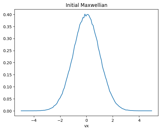
v1_bins = sim.f.kinetic_ions.v1_density.grid_v1
f_v1_init = sim.f.kinetic_ions.v1_density.f_binned[0]
plt.plot(v1_bins, f_v1_init)
plt.xlabel("vx")
plt.title("Initial Maxwellian")
[12]:
Text(0.5, 1.0, 'Initial Maxwellian')
[13]:
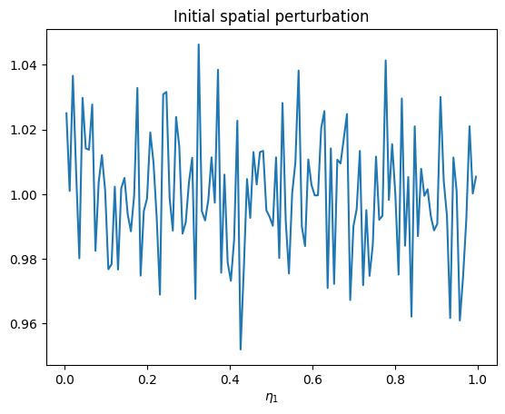
# plot in e1

e1_bins = sim.f.kinetic_ions.e1_density.grid_e1
df_e1_init = sim.f.kinetic_ions.e1_density.delta_f_binned[0]

plt.plot(e1_bins, df_e1_init)
plt.xlabel("$\eta_1$")
plt.title("Initial spatial perturbation")
[13]:
Text(0.5, 1.0, 'Initial spatial perturbation')
[14]:
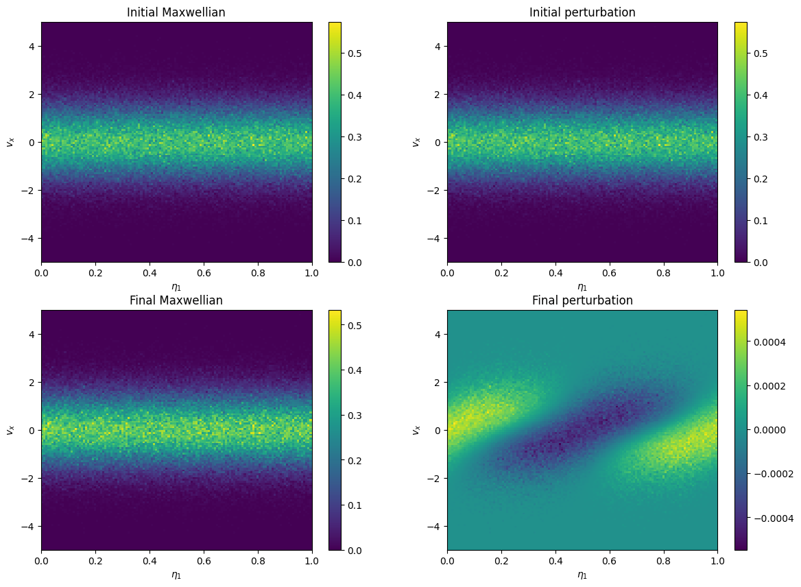
# plot in e1-v1

e1_bins = sim.f.kinetic_ions.e1_v1_density.grid_e1
v1_bins = sim.f.kinetic_ions.e1_v1_density.grid_v1
f_init = sim.f.kinetic_ions.e1_v1_density.f_binned[0]
df_init = sim.f.kinetic_ions.e1_v1_density.delta_f_binned[0]
f_end = sim.f.kinetic_ions.e1_v1_density.f_binned[-1]
df_end = sim.f.kinetic_ions.e1_v1_density.delta_f_binned[-1]

plt.figure(figsize=(14, 10))

plt.subplot(2, 2, 1)
plt.pcolor(e1_bins, v1_bins, f_init.T)
plt.xlabel("$\eta_1$")
plt.ylabel("$v_x$")
plt.title("Initial Maxwellian")
plt.colorbar()

plt.subplot(2, 2, 2)
plt.pcolor(e1_bins, v1_bins, df_init.T)
plt.xlabel("$\eta_1$")
plt.ylabel("$v_x$")
plt.title("Initial perturbation")
plt.colorbar()

plt.subplot(2, 2, 3)
plt.pcolor(e1_bins, v1_bins, f_end.T)
plt.xlabel("$\eta_1$")
plt.ylabel("$v_x$")
plt.title("Final Maxwellian")
plt.colorbar()

plt.subplot(2, 2, 4)
plt.pcolor(e1_bins, v1_bins, df_end.T)
plt.xlabel("$\eta_1$")
plt.ylabel("$v_x$")
plt.title("Final perturbation")
plt.colorbar()
[14]:
<matplotlib.colorbar.Colorbar at 0x7fee579de0e0>
[15]:
# electric field
e1, e2, e3 = sim.grids_log
e_field = sim.spline_values.em_fields.e_field_log
print(e_field)
type(self.data) = <class 'dict'>
len(self.data) = 11
key = np.float64(0.0)    shape = [(257, 9, 9), (257, 9, 9), (257, 9, 9)]
key = np.float64(0.05)   shape = [(257, 9, 9), (257, 9, 9), (257, 9, 9)]
key = np.float64(0.1)    shape = [(257, 9, 9), (257, 9, 9), (257, 9, 9)]
key = np.float64(0.15)   shape = [(257, 9, 9), (257, 9, 9), (257, 9, 9)]
key = np.float64(0.2)    shape = [(257, 9, 9), (257, 9, 9), (257, 9, 9)]
key = np.float64(0.25)   shape = [(257, 9, 9), (257, 9, 9), (257, 9, 9)]
key = np.float64(0.3)    shape = [(257, 9, 9), (257, 9, 9), (257, 9, 9)]
key = np.float64(0.35)   shape = [(257, 9, 9), (257, 9, 9), (257, 9, 9)]
key = np.float64(0.4)    shape = [(257, 9, 9), (257, 9, 9), (257, 9, 9)]
key = np.float64(0.45)   shape = [(257, 9, 9), (257, 9, 9), (257, 9, 9)]
key = np.float64(0.5)    shape = [(257, 9, 9), (257, 9, 9), (257, 9, 9)]
[16]:
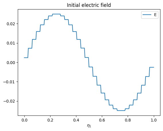
e_vals = e_field.data[0][0]
plt.plot(e1, e_vals[:, 0, 0], label="E")
plt.xlabel("$\eta_1$")
plt.title("Initial electric field")
plt.legend()
[16]:
<matplotlib.legend.Legend at 0x7fee5775e0b0>