
Dev 1 - FEEC boundary conditions#
This tutorial is a first introduction to the use of finite element exterior calculus (FEEC) in Struphy. It is not meant to be a comprehensive introduction to FEEC, but rather a practical guide to how to use it in Struphy. For a more comprehensive introduction to FEEC, see the numerics section of the Struphy doc and the references therein.
Boundary conditions: basics#
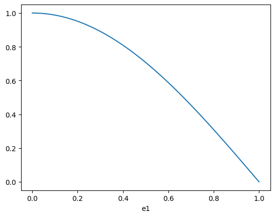
Our first aim is to project a simple function into the H1 and L2 spaces. We will do this for Derham objects with different boundary conditions and plot the results. Here is our function:
[1]:
import numpy as np
from matplotlib import pyplot as plt

fun = lambda e1, e2, e3: np.cos(np.pi/2 * e1)
e1 = np.linspace(0, 1, 100)
e2 = 0.5
e3 = 0.5
plt.plot(e1, fun(e1, e2, e3))
plt.xlabel('e1')
plt.show()
First, create a Derham object with 16 elements in the first direction:
[2]:
from struphy.feec.psydac_derham import Derham
from struphy.topology.grids import TensorProductGrid
from struphy.io.options import DerhamOptions

grid = TensorProductGrid(num_elements=(16, 1, 1))
derham_opts = DerhamOptions()
derham = Derham(grid, derham_opts)
By default, the spline degrees are 1 in each direction:
[3]:
derham.degree
[3]:
(1, 1, 1)
By default, the boundary conditions are periodic in each direction (no boundary conditions):
[4]:
derham.bcs
[4]:
(None, None, None)
Let us apply the geometric projector P0 into the discrete H1 space. The result will be of type StencilVector:
[5]:
vec = derham.P0(fun)
print(type(vec))
<class 'feectools.linalg.stencil.StencilVector'>
The StencilVector is Psydac’s (and thus Struphy’s) fundamental data structure for FE coefficients. It has many attributes and methods attached to it, which will be discussed in more detail in a future tutorial. For now, we will just look at what the .shape method returns, to make clear that this is not just a normal numpy array:
[6]:
print(vec.shape)
print(vec[:].shape)
(np.int64(16),)
(18, 3, 3)
More on StencilVectors later. One convenient method for developers is .toarray(), which converts the StencilVector into a normal numpy array. This is useful for plotting and debugging:
[7]:
vec.toarray()
[7]:
array([1.        , 0.99518473, 0.98078528, 0.95694034, 0.92387953,
       0.88192126, 0.83146961, 0.77301045, 0.70710678, 0.63439328,
       0.55557023, 0.47139674, 0.38268343, 0.29028468, 0.19509032,
       0.09801714])
The StencilVector thus holds FE coefficients. To get a function that we can evaluate at arbitrary points, we can use the create_spline_function method of the Derham object. This creates a callable object that evaluates the FE function at given points:
[8]:
fun_h = derham.create_spline_function(name="hello world",
                                      space_id="H1",
                                      coeffs=vec,
                                      )
plt.plot(e1, fun(e1, e2, e3), label="exact")
plt.plot(e1, fun_h(e1, e2, e3, squeeze_out=True), "r--", label="H1 (periodic)")
plt.xlabel('e1')
plt.legend()
plt.show()
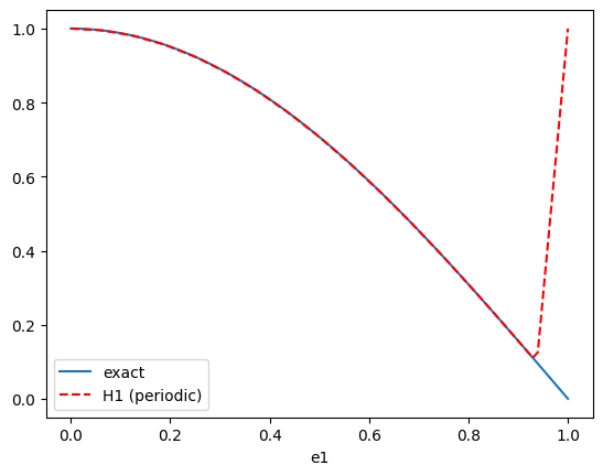
Ooops - something went wrong here! Indeed, the periodic boundary conditions are not compatible with the function we are trying to project. Let us change the boundary conditions to be non-periodic in the first direction, and periodic in the other two:
[9]:
grid = TensorProductGrid(num_elements=(16, 1, 1))
derham_opts = DerhamOptions(bcs=(("dirichlet", "dirichlet"), None, None))
derham = Derham(grid, derham_opts)

vec = derham.P0(fun)
fun_h = derham.create_spline_function(name="hello world",
                                      space_id="H1",
                                      coeffs=vec,
                                      )
plt.plot(e1, fun(e1, e2, e3), label="exact")
plt.plot(e1, fun_h(e1, e2, e3, squeeze_out=True), "r--", label="H1 (dirichlet)")
plt.xlabel('e1')
plt.legend()
plt.show()
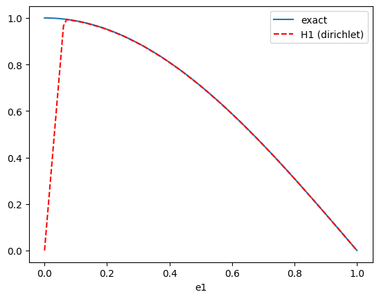
Wrong again! The homogeneous Dirichlet conditions do not respect the non-zero boundary condition on the left. Let us change the boundary condition to be free boundary on the left:
[10]:
grid = TensorProductGrid(num_elements=(16, 1, 1))
derham_opts = DerhamOptions(bcs=(("free", "dirichlet"), None, None))
derham = Derham(grid, derham_opts)
vec = derham.P0(fun)
fun_h = derham.create_spline_function(name="hello world",
                                      space_id="H1",
                                      coeffs=vec,
                                      )
plt.plot(e1, fun(e1, e2, e3), label="exact")
plt.plot(e1, fun_h(e1, e2, e3, squeeze_out=True), "r--", label="H1 (free and dirichlet)")
plt.xlabel('e1')
plt.legend()
plt.show()
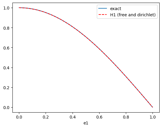
Voilà - that does the job. So far we projected into the discrete H1 space. For comparison, let us also project into the discrete L2 space, with the wrong boundary conditions for illustration purposes:
[11]:
grid = TensorProductGrid(num_elements=(16, 1, 1))
derham_opts = DerhamOptions(bcs=(("dirichlet", "dirichlet"), None, None))
derham = Derham(grid, derham_opts)

vec0 = derham.P0(fun)
vec3 = derham.P3(fun)

fun0_h = derham.create_spline_function(name="hello world H1",
                                      space_id="H1",
                                      coeffs=vec0,
                                      )
fun3_h = derham.create_spline_function(name="hello world L2",
                                      space_id="L2",
                                      coeffs=vec3,
                                      )
plt.plot(e1, fun(e1, e2, e3), label="exact")
plt.plot(e1, fun0_h(e1, e2, e3, squeeze_out=True), "r--", label="H1 (dirichlet)")
plt.plot(e1, fun3_h(e1, e2, e3, squeeze_out=True), "g--", label="L2 (dirichlet)")
plt.xlabel('e1')
plt.legend()
plt.show()
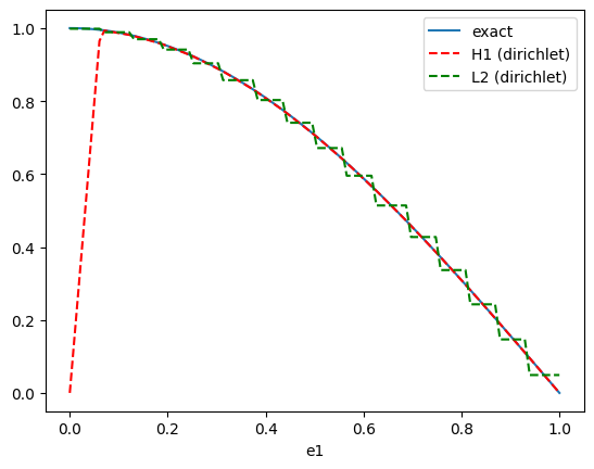
Two things to note here:
The discrete L2 space is less regular (piece-wise constant) than the discrete H1 space (piece-wise linear for degree
p=1).Even though we set the boundary conditions for the whole Derham complex, they are not actually applied to the L2 space, since this space does not have any boundary conditions. This is a common source of confusion for developers new to FEEC, so it is worth pointing out explicitly. It becomes clear when thinking of the 1d Derham sequence: applying the derivative to a function in \(H^1_0\) (with hom. Dirichlet conditions) gives a function in L2. But the derivative of the function in \(H^1_0\) at the boundary can have any value, and is not forced to be zero. This thought applies to any component of a spline function that is a
D-spline: they cannot be set to a specific value.
Neumann boundary conditions#
We solve the 1d Poisson equation
where the source \(\rho\) is given by the function fun defined above. We thus have the exact solution
where \(a\) and \(b\) are constants that depend on the boundary conditions. We will solve this equation with different boundary conditions and compare the numerical solution to the exact solution.
Case \(a = b = 0\):#
[12]:
mfct_solution = lambda e1: 1/(np.pi/2)**2 * np.cos(np.pi/2 * e1)
We start by loading the PDE mode Poisson and by setting fun as the source term:
[13]:
from struphy.models import Poisson

poisson = Poisson()
poisson.propagators.poisson.options = poisson.propagators.poisson.Options(rho=fun)
Next we set up the simulation object with appropriate grid and boundary conditions, then run the simulation for one time step:
[14]:
from struphy import Simulation
from struphy import DerhamOptions, grids

grid = grids.TensorProductGrid(num_elements=(16, 1, 1))
derham_options = DerhamOptions(bcs=(("free", "dirichlet"), None, None))
sim = Simulation(model=poisson,
                 grid=grid,
                 derham_opts=derham_options,
                 )

sim.run(one_time_step=True, verbose=False)
Starting simulation run for model Poisson ...
Struphy run finished.
Post porcessing and loading the plotting data in verbose mode yields:
[15]:
sim.pproc()
sim.load_plotting_data(verbose=True)
100%|██████████| 2/2 [00:00<00:00, 1091.84it/s]
100%|██████████| 2/2 [00:00<00:00, 223.44it/s]
100%|██████████| 2/2 [00:00<00:00, 2223.33it/s]
Let’s extract the grid in eta1 direction (corresponds to the x-direction for the unit cube mapping) and the solution phi:
[16]:
e1h = sim.plotting_data.grids_log[0]
print(e1h)
[0.     0.0625 0.125  0.1875 0.25   0.3125 0.375  0.4375 0.5    0.5625
 0.625  0.6875 0.75   0.8125 0.875  0.9375 1.    ]
[17]:
phi = sim.plotting_data.spline_values.em_fields.phi_log
print(phi)
type(self.data) = <class 'dict'>
len(self.data) = 2
key = np.float64(0.0)    shape = [(17, 2, 2)]
key = np.float64(0.01)   shape = [(17, 2, 2)]
We plot the solution to verify that it matches the exact solution:
[18]:
plt.plot(e1, mfct_solution(e1), label="exact")
plt.plot(e1h, phi.data[0.0][0][:, 0, 0], "go", label="numerical solution")
plt.xlabel('e1')
plt.legend()
[18]:
<matplotlib.legend.Legend at 0x7f0b9f759ea0>
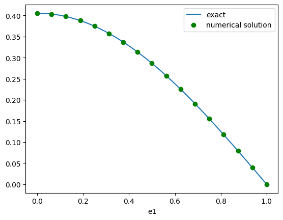
The boundary condition at e1=1.0 was set to dirichlet, which was correctly captured by the solver. The left boundary condition at e1=0.0 was set to free, so how did the solver capture the the Neumann boundary condition? The answer lies in the weak formulation of the problem, which is implemented in the Poisson model: find \(\phi \in H^1\) such that
Note that the left-hand side has been integrated by parts, but that the ensuing boundary term has been ignored:
The boundary term reads
where the second equality follows from the homogeneous Dirichlet condition at e1=1.0, yielding \(v(1)=0\). However, \(v(0)\) is free, so that vanishing of the boundary term implies
This is called a natural boundary condition: it is not explicitly enforced, but rather emerges from the weak formulation of the problem. In contrast, the homogeneous Dirichlet condition at e1=1.0 is an essential boundary condition, which is explicitly enforced by the chosen solution space.
Lifting boundary conditions#
We solve the same problem as above, but with different boundary conditions:
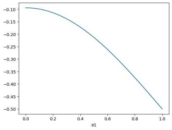
Case \(a = -0.5\), \(b = 0\):#
[19]:
mfct_solution = lambda e1: 1/(np.pi/2)**2 * np.cos(np.pi/2 * e1) - 0.5
[20]:
from struphy.initial.base import GenericPerturbation

tmp = lambda e1, e2, e3: mfct_solution(e1)
fun_lift = GenericPerturbation(tmp)

e1 = np.linspace(0, 1, 100)
e2 = 0.5
e3 = 0.5

plt.plot(e1, fun_lift(e1, e2, e3))
plt.xlabel('e1')
plt.show()
[21]:
grid = grids.TensorProductGrid(num_elements=(16, 1, 1))
derham_options = DerhamOptions(bcs=(("free", "dirichlet"), None, None))

poisson = Poisson()
poisson.propagators.poisson.options = poisson.propagators.poisson.Options(rho=fun)
poisson.em_fields.phi.lifting_function = fun_lift

sim = Simulation(model=poisson,
                 grid=grid,
                 derham_opts=derham_options,
                 )
[22]:
sim.allocate()
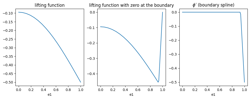
[23]:
var = poisson.em_fields.phi

plt.figure(figsize=(12, 4))
plt.subplot(1, 3, 1)
plt.plot(e1, var.spline_lift(e1, e2, e3, squeeze_out=True))
plt.xlabel('e1')
plt.title("lifting function")

plt.subplot(1, 3, 2)
plt.plot(e1, var.spline_0(e1, e2, e3, squeeze_out=True))
plt.xlabel('e1')
plt.title("lifting function with zero at the boundary")

plt.subplot(1, 3, 3)
plt.plot(e1, var.boundary_spline(e1, e2, e3, squeeze_out=True))
plt.xlabel('e1')
plt.title("$\phi'$ (boundary spline)")

plt.show()
[24]:
print(var.spline.space)
print(var.spline.derham.bcs)
print(var.boundary_spline.space)
print(var.boundary_spline.derham.bcs)
<feectools.linalg.stencil.StencilVectorSpace object at 0x7f0b9e39ff10>
(('free', 'dirichlet'), None, None)
<feectools.linalg.stencil.StencilVectorSpace object at 0x7f0b9e13d5d0>
(('free', 'free'), None, None)