Geometric finite elements (FEEC)

Basics

In conforming finite element (FE) methods, the general principle of approximating a function \(u \in V\) in a space \(V\) is

\[u \approx u_h = \sum_{i=1}^{M} u_i \Lambda_i \quad \in V_h\,,\]

where \(\Lambda_i \in V\) are linearly independent basis functions, \((u_i)_i \in \mathbb R^M\) are called coefficients and \(M \in \mathbb N\) is the dimension of the subspace \(V_h \subset V\) spanned by the basis functions. The thing the differentiates FE methods from spectral methods is the fact that the \(\Lambda_i\) have local support around some grid point \(x_i\). A nice feature of FE methods is that \(u_h \in V\), which leads often to an elegant analysis of the method. The implementation of a FE method consists in writing down a system of equations for the coefficients \((u_i)_i \in \mathbb R^M\), leaving the basis functions fixed.

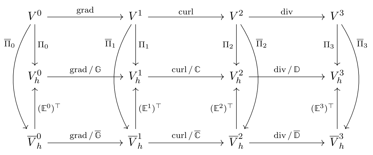
We denote by “geometric finite elements” the FE method based on finite element exterior calculus (FEEC). In 3D, it consists of a sequence of discrete (=finite dimensional) spaces \(V_h^n,\,0\leq n \leq 3\) that satisfy the 3d Derham diagram:

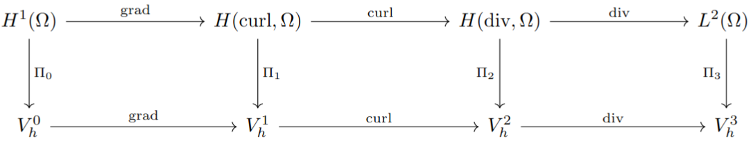
Fig. 1: 3d Derham diagram.

The upper row is a sequence of continuous function spaces, where the last space \(L^2(\Omega)\) is the space of square-integrable functions on \(\Omega\). The other spaces are:

\(H^1(\Omega)\): functions \(f \in L^2(\Omega)\) for which \(\nabla f \in (L^2(\Omega))^3\)

\(H(\textnormal{curl}, \Omega)\): functions \(\mathbf u \in (L^2(\Omega))^3\) for which \(\nabla \times \mathbf u \in (L^2(\Omega))^3\)

\(H(\textnormal{div}, \Omega)\): functions \(\mathbf u \in (L^2(\Omega))^3\) for which \(\nabla \cdot \mathbf u \in L^2(\Omega)\)

More information on these spaces can be found in many textbooks on FE methods, for instance in Brezzi, Fortin, “Mixed and Hybrid Finite Element Methods”.

Struphy uses a conforming” FE method,

\[V_h^0 \subset H^1(\Omega),\qquad V_h^1 \subset H(\textnormal{curl}, \Omega),\qquad V_h^2 \subset H(\textnormal{div}, \Omega),\qquad V_h^3 \subset L^2(\Omega)\]

The operators \(\Pi_n,\,0\leq n \leq 3\) project (\(\Pi_n^2 = \Pi_n\)) into the subspaces :

\[\Pi_0: \, H^1(\Omega) \to V_h^0,\qquad \Pi_1:\, H(\textnormal{curl}, \Omega) \to V_h^1,\qquad \Pi_2:\, H(\textnormal{div}, \Omega) \to V_h^2,\qquad \Pi_3:\, L^2(\Omega) \to V_h^3\]

These spaces and the associated operators of the Derham diagram have been implemented in the open-source package Psydac. Struphy interfaces to this library by means of the class struphy.feec.psydac_derham.Derham.

Both the continuous and the discrete spaces form a complex, which means

\[\textnormal{curl}\,\textnormal{grad} = 0\,,\qquad \textnormal{div}\,\textnormal{curl} = 0\]

holds on both levels. Moreover, the above diagram can be viewed as composed of three commuting diagrams, namely

(1)\[\Pi_1\textnormal{grad} = \textnormal{grad}\,\Pi_0\,,\qquad \Pi_2\textnormal{curl} = \textnormal{curl}\,\Pi_1\,,\qquad \Pi_3\textnormal{div} = \textnormal{div}\,\Pi_2\]

In Struphy the discrete spaces \(V_h^n,\,0\leq n \leq 3\) are spanned by tensor-product B-spline basis functions. Building blocks are the Uni-variate spline spaces of degree \(p\) with basis functions \(N^p(\eta)\) and \(D^{p -1}(\eta)\) defined on the unit interval \(\eta \in [0, 1]\). Hence, in Struphy the simualtion domain is always the unit cube, \((\eta_1,\eta_2,\eta_3) \in \Omega = [0, 1]^3\). The tensor-product basis functions are denoted as follows:

\begin{align} \Lambda^0_{ijk}(\eta_1,\eta_2,\eta_3) &= N_i^{p_1}(\eta_1) N_j^{p_2}(\eta_2) N_k^{p_3}(\eta_3)\,,\qquad &&\mathbf \Lambda^0 = (\Lambda^0_{ijk})_{i=1, j=1, k=1}^{n_1, n_2, n_3} \qquad \\\\ \vec{\Lambda}^1_{1,ijk}(\eta_1,\eta_2,\eta_3) &= \begin{pmatrix} D_i^{p_1 - 1}(\eta_1) N_j^{p_2}(\eta_2) N_k^{p_3}(\eta_3) \\ 0 \\ 0 \end{pmatrix}\,,\qquad &&\vec{\mathbf \Lambda}^1_1 = (\vec \Lambda^1_{1,ijk})_{i=1, j=1, k=1}^{d_1, n_2, n_3} \\\\ \vec{\Lambda}^1_{2,ijk}(\eta_1,\eta_2,\eta_3) &= \begin{pmatrix} 0 \\ N_i^{p_1}(\eta_1) D_j^{p_2 - 1}(\eta_2) N_k^{p_3}(\eta_3) \\ 0 \end{pmatrix}\,,\qquad &&\vec{\mathbf \Lambda}^1_2 = (\vec \Lambda^1_{2,ijk})_{i=1, j=1, k=1}^{n_1, d_2, n_3} \\\\ \vec{\Lambda}^1_{3,ijk}(\eta_1,\eta_2,\eta_3) &= \begin{pmatrix} 0 \\ 0 \\ N_i^{p_1}(\eta_1) N_j^{p_2}(\eta_2) D_k^{p_3 - 1}(\eta_3) \end{pmatrix}\,,\qquad &&\vec{\mathbf \Lambda}^1_3 = (\vec \Lambda^1_{3,ijk})_{i=1, j=1, k=1}^{n_1, n_2, d_3} \\\\ \vec{\Lambda}^2_{1,ijk}(\eta_1,\eta_2,\eta_3) &= \begin{pmatrix} N_i^{p_1}(\eta_1) D_j^{p_2 - 1}(\eta_2) D_k^{p_3 - 1}(\eta_3) \\ 0 \\ 0 \end{pmatrix}\,,\qquad &&\vec{\mathbf \Lambda}^2_1 = (\vec \Lambda^2_{1,ijk})_{i=1, j=1, k=1}^{n_1, d_2, d_3} \\\\ \vec{\Lambda}^2_{2,ijk}(\eta_1,\eta_2,\eta_3) &= \begin{pmatrix} 0 \\ D_i^{p_1 - 1}(\eta_1) N_j^{p_2}(\eta_2) D_k^{p_3 - 1}(\eta_3) \\ 0 \end{pmatrix}\,,\qquad &&\vec{\mathbf \Lambda}^2_2 = (\vec \Lambda^2_{2,ijk})_{i=1, j=1, k=1}^{d_1, n_2, d_3} \\\\ \vec{\Lambda}^2_{3,ijk}(\eta_1,\eta_2,\eta_3) &= \begin{pmatrix} 0 \\ 0 \\ D_i^{p_1 - 1}(\eta_1) D_j^{p_2 - 1}(\eta_2) N_k^{p_3}(\eta_3) \end{pmatrix}\,,\qquad &&\vec{\mathbf \Lambda}^2_3 = (\vec \Lambda^2_{3,ijk})_{i=1, j=1, k=1}^{d_1, d_2, n_3} \\\\ \Lambda^3_{ijk}(\eta_1,\eta_2,\eta_3) &= D_i^{p_1 - 1}(\eta_1) D_j^{p_2 - 1}(\eta_2) D_k^{p_3 - 1}(\eta_3)\,,\qquad &&\mathbf \Lambda^3 = (\Lambda^3_{ijk})_{i=1, j=1, k=1}^{d_1, d_2, d_3} \qquad \end{align}

Elements of the discrete spaces are linear combinations of the respective basis functions:

\begin{align} V_h^0 &= \textnormal{span}(\mathbf \Lambda^0)\,,\qquad p_h^0(\eta_1,\eta_2,\eta_3) = \sum_{ijk} p_{ijk}\, \Lambda^0_{ijk}(\eta_1,\eta_2,\eta_3) = \mathbf p^\top \mathbf \Lambda^0 \quad \in \,V_h^0 \\ V_h^1 &= \textnormal{span}(\vec{\mathbf \Lambda}^1_1, \vec{\mathbf \Lambda}^1_2, \vec{\mathbf \Lambda}^1_3)\,, \\ &\qquad\qquad \mathbf E_h^1(\eta_1,\eta_2,\eta_3) = \sum_{\mu=1}^3 \sum_{ijk} e_{\mu, ijk}\,\vec{\Lambda}^1_{\mu, ijk}(\eta_1,\eta_2,\eta_3) = \sum_{\mu=1}^3 \mathbf e_\mu^\top \vec{\mathbf \Lambda}^1_\mu = \mathbf e^\top \vec{\mathbf \Lambda}^1 \quad \in \,V_h^1 \\ V_h^2 &= \textnormal{span}(\vec{\mathbf \Lambda}^2_1, \vec{\mathbf \Lambda}^2_2, \vec{\mathbf \Lambda}^2_3)\,, \\ &\qquad \qquad \mathbf B_h^2(\eta_1,\eta_2,\eta_3) = \sum_{\mu=1}^3 \sum_{ijk} b_{\mu, ijk}\,\vec{\Lambda}^2_{\mu, ijk}(\eta_1,\eta_2,\eta_3) = \sum_{\mu=1}^3 \mathbf b_\mu^\top \vec{\mathbf \Lambda}^2_\mu = \mathbf b^\top \vec{\mathbf \Lambda}^2 \quad \in \,V_h^2 \\ V_h^3 &= \textnormal{span}(\mathbf \Lambda^3)\,,\qquad n_h^3(\eta_1,\eta_2,\eta_3) = \sum_{ijk}^{\phantom{3}} n_{ijk}\, \Lambda^3_{ijk}(\eta_1,\eta_2,\eta_3) = \mathbf n^\top \mathbf \Lambda^3 \quad \in \,V_h^3 \end{align}

The discrete spline functions are represented by their FE coefficients \(\mathbf p \in \mathbb R^{N_0}\), \(\mathbf e \in \mathbb R^{N_1}\), \(\mathbf b \in \mathbb R^{N_2}\) and \(\mathbf n \in \mathbb R^{N_3}\). The class for callable spline functions in Struphy is struphy.feec.derham.SplineFuntion. In particular, each SplineFuntion object has

1. the property vector holding the FE coefficients, along with a setter method,

2. a __call__() method for evaluating the spline at (an array of) points \((\eta_{ijk})_{ijk}\).

A splien function can be created via the factory function struphy.feec.derham.Derham.create_spline_function(). The space dimensions are products of the uni-variate dimensions:

\begin{align} \textnormal{dim} V_h^0 &= N_0 = n_1 n_2 n_3 \\\\ \textnormal{dim} V_h^1 &= N_1 = d_1 n_2 n_3 + n_1 d_2 n_3 + n_1 n_2 d_3 \\\\ \textnormal{dim} V_h^2 &= N_2 = n_1 d_2 d_3 + d_1 n_2 d_3 + d_1 d_2 n_3 \\\\ \textnormal{dim} V_h^3 &= N_3 = d_1 d_2 d_3 \end{align}

The derivatives act as follows on the FE coefficients:

\begin{align} \textnormal{grad}\, p_h^0 &= (\mathbb G \mathbf p)^\top \vec{\mathbf \Lambda}^1 \quad \in \,V_h^1 \\\\ \textnormal{curl}\, \mathbf E_h^1 &= (\mathbb C \mathbf e)^\top \vec{\mathbf \Lambda}^2 \quad \in \,V_h^2 \\\\ \textnormal{div}\, \mathbf B_h^2 &= (\mathbb D \mathbf b)^\top \mathbf \Lambda^3 \quad \in \,V_h^3 \end{align}

Here, we introduced the discrete linear operators \(\mathbb G: \mathbb R^{N_0} \to \mathbb R^{N_1}\), \(\mathbb C: \mathbb R^{N_1} \to \mathbb R^{N_2}\) and \(\mathbb D: \mathbb R^{N_2} \to \mathbb R^{N_3}\), which satisfy the complex property

\[\mathbb C\, \mathbb G = 0\,,\qquad \mathbb D\, \mathbb C = 0\]

Note

A struphy userguide for the operators \(\mathbb G\), \(\mathbb C\) and \(\mathbb D\) and for the projection operators \(\Pi_n\) is given in this Jupyter notebook.

The projectors \(\Pi_n,\, 0\leq n \leq 3\) into the discrete spaces \(V_h^n,\, 0\leq n \leq 3\) are constructed such that the commuting relations (1) hold. They are defined by Degrees of freedom (DOFs) \(\sigma^n,\, 0\leq n \leq 3\) which are functionals that map continuous functions to real numbers. The number of DOFs for each space is equal to its dimension. A common DOF is the evaluation of a function at a certain point in \(\Omega\); if we choose \(N_0\) such distinct points and call the corresponding DOFs \((\sigma^0_{ijk})_{i=1,j=1, k=1}^{n_1,n_2,n_3}\), we can define a projector \(\Pi_0:H^1 \to V_h^0\) by

(2)\[\sigma^0_{ijk}(p_h^0) = \sigma^0_{ijk}(p^0)\,,\qquad p^0 \in H^1 \mapsto p_h^0 \in V_h^0\]

These are \(N_0\) equations for the coefficients \(\mathbf p \in \mathbb R^{N_0}\) of \(p_h^0 \in V_h^0\). The above formula is nothing else than classical interpolation and is used for the \(\Pi_0\)-projector in Struphy. The other projectors are a mix of interpolation and “histopolation” (integration between two interpolation points), as depicted in Fig. 2. For instance, to project into the space \(V_h^1\) (1-form), the first component is “histopolated” in \(\eta_1\)-direction (orange lines) and interpolated in \((\eta_2, \eta_3)\) (blue points); the second component is “histopolated” in \(\eta_2\)-direction and interpolated in \((\eta_1, \eta_3)\); the third component is “histopolated” in \(\eta_3\)-direction and interpolated in \((\eta_1, \eta_2)\). The DOFs for \(V_h^2\) contain histopolation over surface elements (green) and for \(V_h^3\) one has 3d histopolation over volume elements (violet). This ultimately leads to the commuting property.

Fig. 2: Degrees of freedom (DOFs) of the commuting projectors.

Uni-variate spline spaces

Finite element spaces in Struphy are based on uni-variate B-spline spaces on the interval \(\eta \in [0, 1]\), as introduced for instance in Section 2.2 of Hughes, Cottrell, Bazilevs, “Isogeometric analysis: CAD, finite elements, NURBS, exact geometry and mesh refinement”, Comput. Methods Appl. Mech. Engrg. 194 (2005). B-spline basis functions of degree \(p\) are denoted by \(N_i^p(\eta)\) (thus also called N-splines in the following). They are piece-wise polynomials with a regularity of at most \(p-1\) (they are piece-wise constants for \(p=0\)). Linear combinations af these basis functions give a spline function

\[f_h(\eta) = \sum_{i=0}^{n-1} f_i N^p_i(\eta)\,,\qquad f_i \in \mathbb R\,,\]

where the \(\mathbf f = (f_i)_{i=0}^{n-1} \in \mathbb R^n\) are the spline coefficients. The dimension of the spline space is \(n\). In Struphy two different boundary conditions can be chosen: periodic or clamped. For the latter, the first and last basis functions are “interpolatory” at \(\eta=0\) and \(\eta=1\), respectively, meaning that \(f_h(0) = f_0\) and \(f_h(1) = f_{n-1}\). Assuming that the interval \([0, 1]\) is split into \(Nel\) cells (or elements), the dimension of the periodic space is \(n=Nel\), whereas the dimension of the clamped space is \(n=Nel + p\). Spline basis functions of degree \(p=2\) are potted in Fig. 3 for \(Nel=8\) cells.

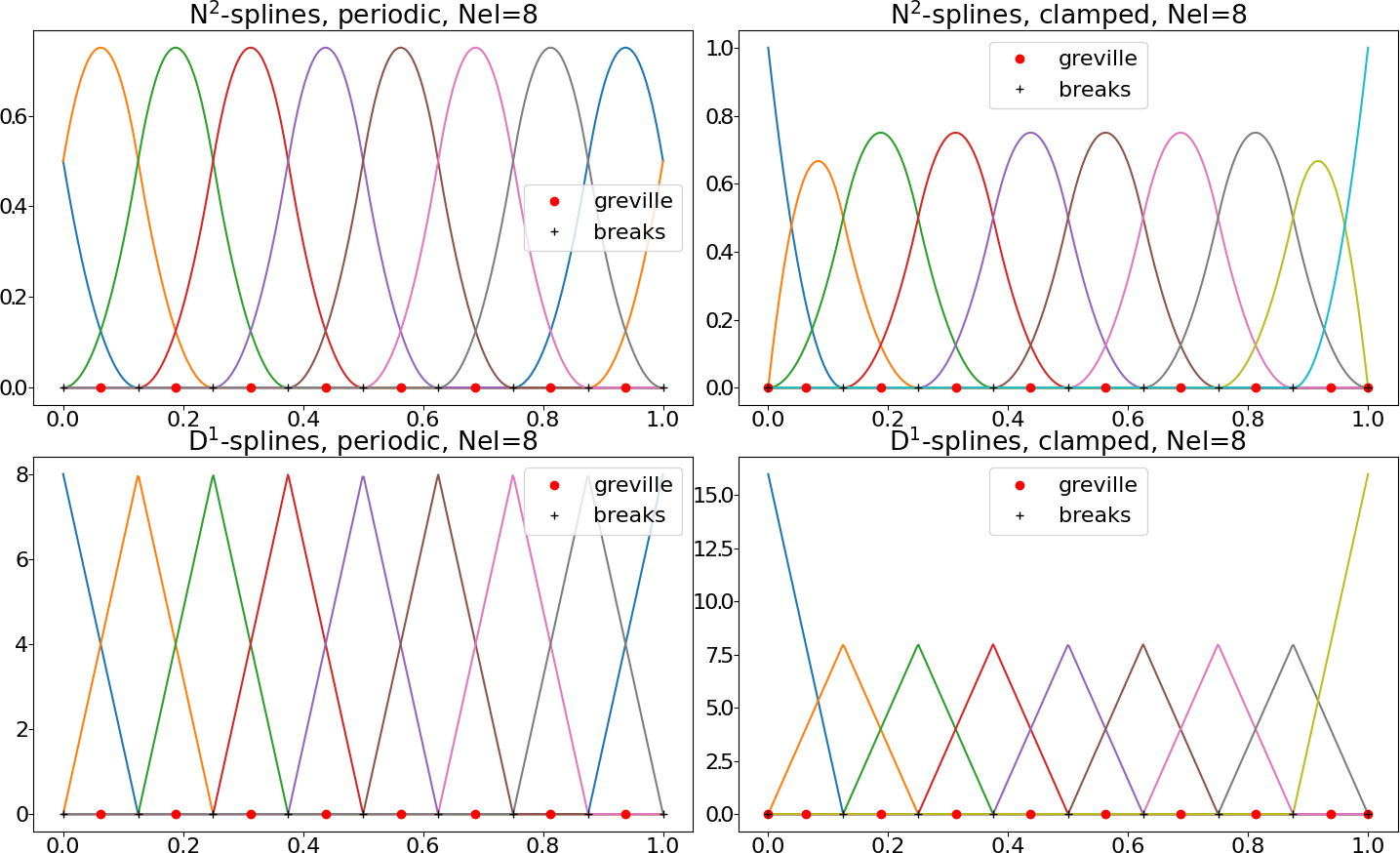
Fig. 3: Uni-variate spline spaces of degree \(p=2\).

In Fig. 3 the black crosses are the break points (cell interfaces) and the red dots are the Greville points, which are the interpolation points used to define the DOFs for the projectors in (2). Moreover, we encounter the so-called D-splines which are related to the derivatives of N-splines via

\[\frac{\partial }{\partial \eta} N_i^p = D^{p-1}_{i-1} - D^{p-1}_i\]

D-splines are rescaled B-splines of degree \(p-1\). In the clamped case the dimension \(d\) of the D-spline space is thus one less than that of N-splines; in this case \(D^{p-1}_{-1} = D^{p-1}_{n-1} = 0\), where \(n\) is the dimension of the N-spline space.

Fig. 4 shows the uni-variate spline spaces for degree \(p=1\). Note that in this case the D-Splines are piece-wise constants and a spline function is therefore generally not continuous.

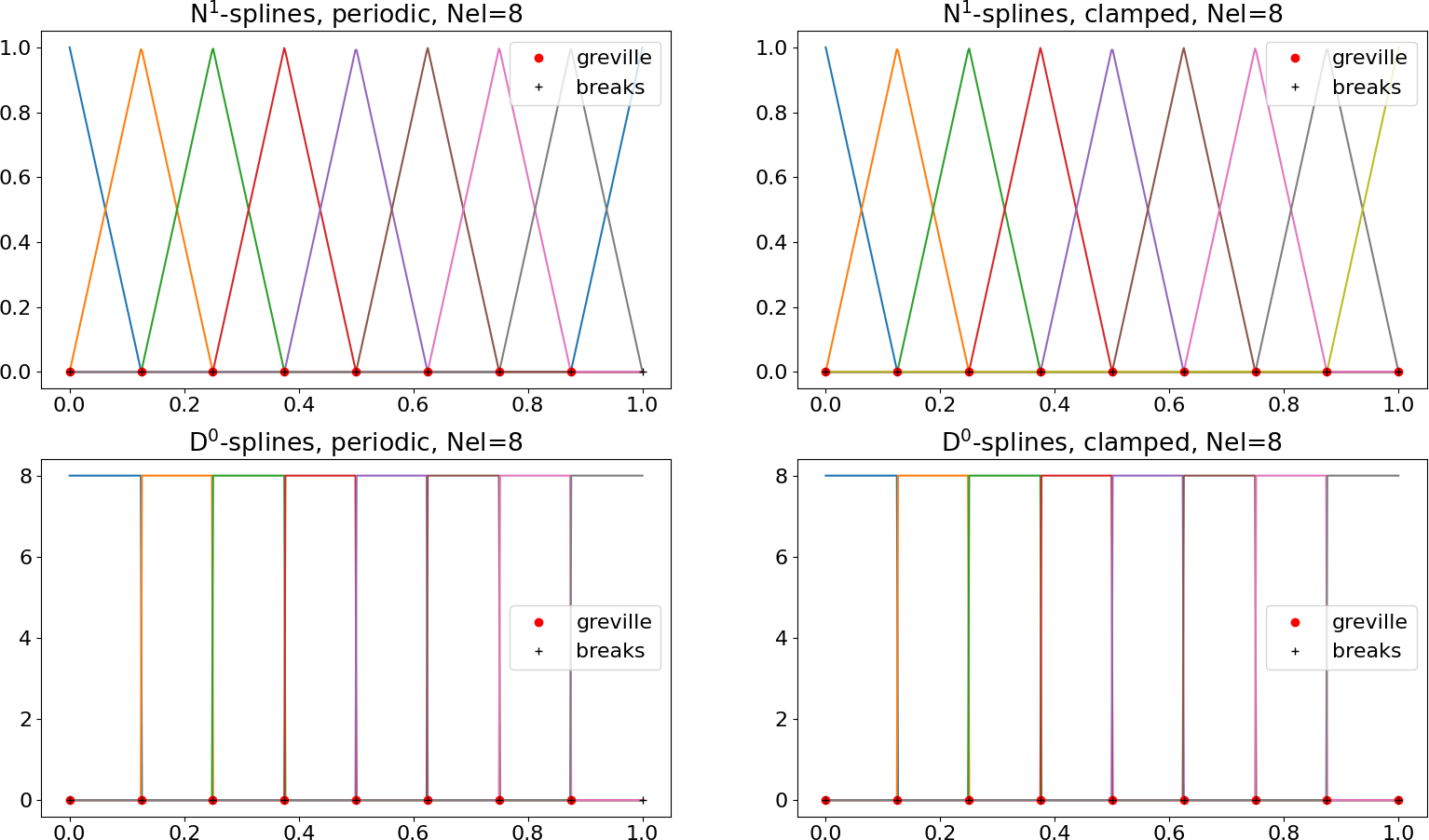
Fig. 4: Uni-variate spline spaces of degree \(p=1\).

Higher degree leads to higher smoothness in Struphy, where spline functions have the maximal regularity \(p-1\). Moreover, the support of each basis function is the union of \(p+1\) adjacent cells and thus increases with the degree. This allows for high-order methods in Struphy. See Fig. 5 for an example with \(p=4\).

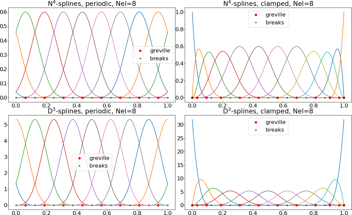
Fig. 4: Uni-variate spline spaces of degree \(p=4\).

Polar splines

Coming soon !