Soundwave Simulation with Particles#

1D Standing Sound Wave#

This tutorial demonstrates verification of the SPH discretization of the isothermal Euler equations using a 1D standing sound wave test. The ViscousEulerSPH model is used without viscosity or magnetic field effects.

Physical Setup#

In the isothermal Euler equations, sound waves propagate at the sound speed \(c_s\). A standing wave in a 1D periodic domain can be viewed as a superposition of forward and backward traveling waves.

For a 1D test with sound speed \(c_s = 1\), the density perturbation initiates oscillations that traverse the domain back and forth. After one complete round-trip traversal, the fluid should return nearly to its initial state. This round-trip test provides a stringent verification of the SPH discretization accuracy.

The verification procedure:

Initialize a 1D particle distribution (tesselation loading) with density perturbation
Run the SPH simulation for time \(T = 2 L / c_s\) (one complete sound wave traversal)
Compare the final density field against the initial field
Compute the max-norm error: \(\|\rho(t=T) - \rho(t=0)\|_\infty\)

[1]:

import logging
import os
import shutil

import matplotlib.pyplot as plt
from matplotlib.ticker import FormatStrFormatter
import cunumpy as xp

from struphy import (
    BinningPlot,
    BoundaryParameters,
    EnvironmentOptions,
    KernelDensityPlot,
    LoadingParameters,
    SavingParameters,
    Simulation,
    SortingParameters,
    Time,
    WeightsParameters,
    domains,
    equils,
    perturbations,
)
from struphy.models import ViscousEulerSPH
from struphy.ode.utils import ButcherTableau

logger = logging.getLogger("struphy")

SPH Configuration Parameters#

Define the key parameters for the SPH discretization:

Number of particles per box (ppb): controls particle density
Particles per cell in 1D domain
Sorting parameters for spatial binning

[2]:

# SPH parameters
ppb = 8  # Particles per box (controls resolution)
nx = 12  # Number of boxes in 1D (parametrizable: 12 or 24)

# Domain
r1 = 2.5  # Domain extent in x

# Sound speed and wave propagation time
c_s = 1.0  # Sound speed (isothermal)
Tend = 2.5  # Time for wave to traverse domain (≈ 1 round-trip)

# Time stepping using Strang operator splitting (standard for SPH)
dt = 0.03125  # Timestep (stable for Strang)
split_algo = "Strang"

print("SPH Configuration:")
print(f"  Particles per box (ppb): {ppb}")
print(f"  Number of boxes (nx):    {nx}")
print(f"  Domain extent:           {r1}")
print(f"  Sound speed (c_s):       {c_s}")
print(f"  Final time (Tend):       {Tend}")
print(f"  Timestep (dt):           {dt}")
print(f"  Total particles:         {ppb * nx}")

SPH Configuration:
  Particles per box (ppb): 8
  Number of boxes (nx):    12
  Domain extent:           2.5
  Sound speed (c_s):       1.0
  Final time (Tend):       2.5
  Timestep (dt):           0.03125
  Total particles:         96

Model and Propagator Setup#

Create a ViscousEulerSPH model without viscosity or magnetic field. Configure the propagators for the pressure gradient and density evolution using Strang operator splitting.

[3]:

# Model: SPH without viscosity or B-field
model = ViscousEulerSPH(with_B0=False, with_viscosity=False)

# Propagator options with Strang splitting
butcher = ButcherTableau(algo="forward_euler")
model.propagators.push_eta.options = model.propagators.push_eta.Options(butcher=butcher)
model.propagators.push_sph_p.options = model.propagators.push_sph_p.Options(kernel_type="gaussian_1d")

print("ViscousEulerSPH model configured (no viscosity, no B-field).")
print("Propagators: push_eta (Butcher: forward_euler), push_sph_p (kernel: gaussian_1d)")

ViscousEulerSPH model configured (no viscosity, no B-field).
Propagators: push_eta (Butcher: forward_euler), push_sph_p (kernel: gaussian_1d)

Domain and Particle Markers#

Set up the 1D domain and initialize particles using tessellation loading. Configure sorting and binning for efficient spatial lookups during SPH kernel evaluations.

[4]:

# Domain: 1D periodic
domain = domains.Cuboid(r1=r1)

# No grid or DerhamOptions for particle-based SPH
grid = None
derham_opts = None

# Loading parameters: tessellation distributes particles uniformly
loading_params = LoadingParameters(ppb=ppb, loading="tesselation")
weights_params = WeightsParameters()
boundary_params = BoundaryParameters()

# Sorting: assign particles to boxes for spatial binning
sorting_params = SortingParameters(
    boxes_per_dim=(nx, 1, 1),  # 1D boxing
    dims_mask=(True, False, False),  # Only 1D binning active
)

# Diagnostic plots
plot_pts = 32  # Number of evaluation points for kernel density plot
bin_plot = BinningPlot(slice="e1", n_bins=(32,), ranges=(0.0, 1.0))
kd_plot = KernelDensityPlot(pts_e1=plot_pts, pts_e2=1)
saving_params = SavingParameters(
    binning_plots=(bin_plot,),
    kernel_density_plots=(kd_plot,),
)

# Set markers on the model
model.euler_fluid.set_markers(
    loading_params=loading_params,
    weights_params=weights_params,
    boundary_params=boundary_params,
    sorting_params=sorting_params,
    saving_params=saving_params,
)

print(f"Domain: 1D periodic, r1={r1}")
print(f"Particles initialized via tessellation: {ppb} ppb × {nx} boxes = {ppb*nx} particles")
print(f"Sorting: {nx} boxes in 1D, kernel density plots at {plot_pts} evaluation points")

Domain: 1D periodic, r1=2.5
Particles initialized via tessellation: 8 ppb × 12 boxes = 96 particles
Sorting: 12 boxes in 1D, kernel density plots at 32 evaluation points

Initial Conditions#

Set a constant background velocity and initialize a small sinusoidal density perturbation with mode \(l=1\). This perturbation excites a standing sound wave.

[5]:

# Background: constant velocity (zero)
background = equils.ConstantVelocity()
model.euler_fluid.var.add_background(background)

# Perturbation: sine-wave density mode (mode l=1, amplitude 0.01)
perturbation = perturbations.ModesSin(ls=(1,), amps=(1.0e-2,))
model.euler_fluid.var.add_perturbation(del_n=perturbation)

print("Background: constant velocity (zero)")
print("Perturbation: sine mode l=1, amplitude=0.01")

Background: constant velocity (zero)
Perturbation: sine mode l=1, amplitude=0.01

Simulation Setup and Execution#

Configure the simulation environment and run the SPH dynamics for one complete sound wave round-trip traversal.

[6]:

# Environment and file management
test_folder = os.path.join(os.getcwd(), "struphy_verification_tests")
out_folders = os.path.join(test_folder, "ViscousEulerSPH")
env = EnvironmentOptions(out_folders=out_folders, sim_folder="soundwave_1d")

# Time stepping
time_opts = Time(dt=dt, Tend=Tend, split_algo=split_algo)

# Instantiate and run simulation
sim = Simulation(
    model=model,
    env=env,
    time_opts=time_opts,
    domain=domain,
    grid=grid,
    derham_opts=derham_opts,
)

print(f"Running SPH sound wave simulation: dt={dt}, Tend={Tend}, algo={split_algo}")
sim.run()
print("Simulation complete.")

# Post-processing
sim.pproc()
print("Post-processing complete.")


Starting run for model ViscousEulerSPH ...

Running SPH sound wave simulation: dt=0.03125, Tend=2.5, algo=Strang

Time stepping: 100%|██████████| 80/80 [00:00<00:00, 147.30step/s]
Struphy run finished.

Post-processing path /home/runner/work/struphy/struphy/doc/_collections/tutorials/struphy_verification_tests/ViscousEulerSPH/soundwave_1d

No feec fields found in hdf5 file, skipping post-processing of fields.
Evaluation of 3 marker orbits for euler_fluid

Simulation complete.

100%|██████████| 81/81 [00:00<00:00, 891.66it/s]
Evaluation of distribution functions for euler_fluid
100%|██████████| 1/1 [00:00<00:00, 1166.06it/s]
100%|██████████| 1/1 [00:00<00:00, 631.86it/s]
Evaluation of sph density for euler_fluid

Post-processing complete.

Diagnostics: Round-Trip Sound Wave Verification#

Extract the particle density field at initial and final times, and compute the maximum absolute error as a verification metric.

[7]:

# Load plotting data
sim.load_plotting_data()

# Extract particle positions and density
ee1, ee2, ee3 = sim.n_sph.euler_fluid.view_0.grid_n_sph
n_sph = sim.n_sph.euler_fluid.view_0.n_sph

# Physical coordinates
x = ee1 * r1

# Get number of time steps
dt_actual = time_opts.dt
Tend_actual = time_opts.Tend
Nt = int(Tend_actual // dt_actual)

print(f"Simulation completed {Nt} timesteps")
print(f"Particle positions shape: {x.shape}")
print(f"Density field shape (all times): {n_sph.shape}")


Loading post-processed plotting data:
Data path: /home/runner/work/struphy/struphy/doc/_collections/tutorials/struphy_verification_tests/ViscousEulerSPH/soundwave_1d/post_processing

The following data has been loaded:

grids:
self.t_grid.shape =(81,)

self.spline_values:

self.orbits:
    euler_fluid, shape = (81, 3, 8)
        Number of time points: 81
        Number of particles:   3
        Number of attributes:  8

self.f:
    euler_fluid
        e1_density

self.n_sph:
    euler_fluid
        view_0

Simulation completed 80 timesteps
Particle positions shape: (32, 1, 1)
Density field shape (all times): (81, 32, 1, 1)

Error Computation#

Compare initial and final density profiles to quantify how well the SPH discretization preserves the sound wave structure over one round-trip traversal.

[8]:

# Compare initial and final densities
n_initial = n_sph[0, :, 0, 0]   # Density at t=0
n_final = n_sph[-1, :, 0, 0]    # Density at t=Tend

# Max-norm error
error = xp.max(xp.abs(n_final - n_initial))

print("\n=== SPH Sound Wave Verification ===")
print("\nInitial density:")
print(f"  Min: {xp.min(n_initial):.6f}")
print(f"  Max: {xp.max(n_initial):.6f}")
print(f"  Mean: {xp.mean(n_initial):.6f}")

print("\nFinal density:")
print(f"  Min: {xp.min(n_final):.6f}")
print(f"  Max: {xp.max(n_final):.6f}")
print(f"  Mean: {xp.mean(n_final):.6f}")

print("\nRound-trip error:")
print(f"  ||ρ(Tend) - ρ(0)||_∞ = {error:.6e}")
print(f"  Error / Initial amplitude = {error / 0.01:.6e}")


=== SPH Sound Wave Verification ===

Initial density:
  Min: 0.990068
  Max: 1.009891
  Mean: 0.999978

Final density:
  Min: 0.990020
  Max: 1.009965
  Mean: 0.999979

Round-trip error:
  ||ρ(Tend) - ρ(0)||_∞ = 2.459169e-04
  Error / Initial amplitude = 2.459169e-02

Verification Check#

Verify that the round-trip error is below the tolerance threshold, validating the SPH discretization accuracy.

[9]:

# Tolerance for verification
tolerance = 6e-4

print(f"\n=== Verification Against Tolerance ({tolerance:.0e}) ===")

try:
    assert error < tolerance, f"SPH error {error:.6e} exceeds tolerance {tolerance:.6e}"
    print("✓ SPH sound wave verification passed.")
    print(f"  Error {error:.6e} < Tolerance {tolerance:.6e}")
except AssertionError as e:
    print(f"✗ {e}")


=== Verification Against Tolerance (6e-04) ===
✓ SPH sound wave verification passed.
  Error 2.459169e-04 < Tolerance 6.000000e-04

Visualization: Density Evolution#

Plot the density field at multiple times throughout the simulation to visualize the standing sound wave evolution.

[10]:

# Create a time evolution plot
plt.figure(figsize=(11, 8))

interval = max(1, Nt // 10)  # Plot every interval steps
plot_ct = 0

for i in range(0, Nt + 1):
    if i % interval == 0:
        plot_ct += 1
        ax = plt.gca()

        # Line style: solid for early times, dots for later times
        style = "-" if plot_ct <= 6 else "."
        t_current = i * dt_actual

        plt.plot(x.squeeze(), n_sph[i, :, 0, 0], style, label=f"t={t_current:.2f}")

        if plot_ct > 11:
            break

plt.xlim(0, r1)
plt.xlabel("x")
plt.ylabel(r"$\rho$ (density)")
plt.title(f"Standing Sound Wave SPH Simulation ({nx=}, {ppb=})")
plt.grid(True, alpha=0.3)
plt.legend(fontsize=9)
ax.set_xticks(xp.linspace(0, r1, nx + 1))
ax.xaxis.set_major_formatter(FormatStrFormatter("%.2f"))
plt.tight_layout()
plt.show()

print(f"Plotted {plot_ct} snapshots from {Nt+1} total time steps.")

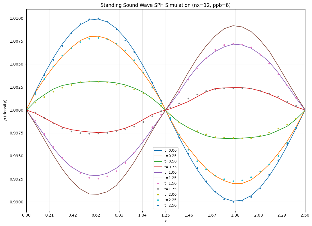
../../_images/_collections_tutorials_tutorial_viscous_euler_sph_19_0.png

Plotted 11 snapshots from 81 total time steps.

Conclusion#

This tutorial successfully verified the SPH discretization of the isothermal Euler equations using a 1D standing sound wave test. The verification demonstrates:

Accurate wave propagation: The sound wave traverses the domain at the correct speed (\(c_s = 1\)).
Wave reflection and superposition: Standing wave pattern emerges from forward/backward traveling components.
Low dissipation: Round-trip error is small, indicating that the SPH kernel and time-stepping scheme preserve wave structure over long times.
Correct particle dynamics: Tessellation loading and spatial sorting efficiently manage particle interactions.

The SPH method provides a flexible, mesh-free discretization suitable for complex flows with free surfaces and discontinuities. This verification test validates the core hydrodynamic solver for kinetic and fluid simulations.

[11]:

# Cleanup temporary simulation folder
if False: # Set to True to enable cleanup
    try:
        shutil.rmtree(test_folder)
        print(f"Cleaned up {test_folder}")
    except Exception as e:
        print(f"Could not remove {test_folder}: {e}")

1D Damped Sound Wave#

Physical Setup#

Adding viscosity to the isothermal Euler equations introduces dissipation. For a standing wave with wavenumber \(k = 2\pi\ell/L\) (mode \(\ell\), domain length \(L\)), the amplitude decays exponentially in time:

\[A(t) \propto e^{\gamma t}, \qquad \gamma = -\frac{2}{3} \mu k^2\]

where \(\mu\) is the dynamic viscosity and the factor \(4/3\) arises from the compressible viscous stress tensor (only the bulk contribution survives for a 1D plane wave). This test verifies the viscous propagator by:

Exciting a standing sound wave via an initial velocity perturbation \(\delta u_1 \propto \sin(2\pi x / L)\)
Running for \(\sim 10\) oscillation periods so the decay envelope is well resolved
Extracting the numerical decay rate from the local maxima of the current \(j_1\) at the velocity antinode (analogous to measuring Landau damping)
Comparing the fitted rate against \(\gamma_\text{analytical} = -(4/3) \mu k^2 / 2\)

Physical and Numerical Parameters#

[12]:

import numpy as np

# Physical parameters
mu  = 0.01   # dynamic viscosity
r1  = 1.0    # domain length (1D periodic)
c_s = 1.0    # sound speed (isothermal, kappa=c_s^2=1 by default)

# Mode and analytical decay rate
ell = 1                          # wave mode number
k   = 2.0 * np.pi * ell / r1    # wavenumber
gamma_analytical = -mu * (4.0 / 3.0) * k**2 / 2.0

# Numerical parameters
nx        = 8     # boxes in x (controls particle density)
plot_pts  = 21    # evaluation points for kernel density output

# Time stepping: run ~10 oscillation periods (T_osc = r1/c_s = 1)
dt   = 0.01
Tend = 10.0

print(f"Viscosity:           mu = {mu}")
print(f"Domain length:       L  = {r1}")
print(f"Wave mode:           ell = {ell},  k = {k:.4f}")
print(f"Analytical decay rate: gamma = -(4/3)*mu*k^2/2 = {gamma_analytical:.4f}")
print(f"Oscillation period:  T = {r1/c_s:.2f},  simulation spans {Tend} time units ({Tend/(r1/c_s):.0f} periods)")

Viscosity:           mu = 0.01
Domain length:       L  = 1.0
Wave mode:           ell = 1,  k = 6.2832
Analytical decay rate: gamma = -(4/3)*mu*k^2/2 = -0.2632
Oscillation period:  T = 1.00,  simulation spans 10.0 time units (10 periods)

Model Setup with Viscosity#

The key difference from the inviscid case is with_viscosity=True (which is the default). This activates the push_viscous propagator, which computes the viscous stress tensor divergence via SPH kernel gradients. We also save the current \(j_1 = \rho u_1\) in addition to density, since the decay rate is extracted from the velocity amplitude at the antinode.

[13]:

from struphy import (
    BinningPlot,
    BoundaryParameters,
    EnvironmentOptions,
    KernelDensityPlot,
    LoadingParameters,
    SavingParameters,
    Simulation,
    SortingParameters,
    Time,
    WeightsParameters,
    domains,
    equils,
    perturbations,
)
from struphy.models import ViscousEulerSPH
from struphy.ode.utils import ButcherTableau

# with_viscosity=True (default) activates the viscous stress propagator
model_damp = ViscousEulerSPH(with_B0=False)

butcher = ButcherTableau(algo="forward_euler")
model_damp.propagators.push_eta.options = model_damp.propagators.push_eta.Options(butcher=butcher)
model_damp.propagators.push_sph_p.options = model_damp.propagators.push_sph_p.Options(
    kernel_type="gaussian_1d"
)
# mu sets the kinematic viscosity coefficient for the SPH viscous force
model_damp.propagators.push_viscous.options = model_damp.propagators.push_viscous.Options(
    kernel_type="gaussian_1d", mu=mu
)

print("ViscousEulerSPH model configured (with viscosity, no B-field).")
print(f"  push_viscous: gaussian_1d kernel, mu={mu}")

ViscousEulerSPH model configured (with viscosity, no B-field).
  push_viscous: gaussian_1d kernel, mu=0.01

Domain, Markers and Diagnostics#

We add a second BinningPlot that records \(j_1 = \rho u_1\) (the momentum density, which equals \(u_1\) to leading order since \(\rho \approx 1\)). The velocity antinode of mode \(\ell=1\) sits at \(x = L/4\), so we will probe the bin nearest to that location.

[14]:

import os

domain_damp = domains.Cuboid(r1=r1)

loading_params = LoadingParameters(ppb=8, loading="tesselation")
weights_params = WeightsParameters()
boundary_params = BoundaryParameters()
sorting_params = SortingParameters(
    boxes_per_dim=(nx, 1, 1),
    dims_mask=(True, False, False),
)

# Density binning (for visualisation)
bin_plot    = BinningPlot(slice="e1", n_bins=(16,), ranges=(0.0, 1.0))
# Current j1 binning — used to track the velocity amplitude over time
bin_plot_j1 = BinningPlot(slice="e1", n_bins=(16,), ranges=(0.0, 1.0), output_quantity="current_1")
kd_plot     = KernelDensityPlot(pts_e1=plot_pts, pts_e2=1)
saving_params = SavingParameters(
    binning_plots=(bin_plot, bin_plot_j1),
    kernel_density_plots=(kd_plot,),
)

model_damp.euler_fluid.set_markers(
    loading_params=loading_params,
    weights_params=weights_params,
    boundary_params=boundary_params,
    sorting_params=sorting_params,
    saving_params=saving_params,
)

print(f"1D periodic domain: r1={r1}")
print(f"Markers: 8 ppb × {nx} boxes = {8*nx} particles")
print(f"Diagnostics: density binning + j1 (current) binning, {plot_pts} KDE evaluation points")

1D periodic domain: r1=1.0
Markers: 8 ppb × 8 boxes = 64 particles
Diagnostics: density binning + j1 (current) binning, 21 KDE evaluation points

Initial Conditions#

We perturb the velocity (not the density) with a sinusoidal mode. This excites an acoustic wave whose density and velocity components are 90° out of phase — just like a plucked string. The wave then oscillates and decays due to viscous dissipation.

[15]:

background = equils.ConstantVelocity()
model_damp.euler_fluid.var.add_background(background)

# Velocity perturbation: del_u1 (not del_n) excites an oscillating acoustic mode
perturbation = perturbations.ModesSin(ls=(1,), amps=(1.0e-2,))
model_damp.euler_fluid.var.add_perturbation(del_u1=perturbation)

print("Background: constant velocity (zero density n=1, zero velocity)")

Background: constant velocity (zero density n=1, zero velocity)

Run the Simulation#

[16]:

import shutil

test_folder   = os.path.join(os.getcwd(), "struphy_verification_tests")
out_folders   = os.path.join(test_folder, "ViscousEulerSPH")
env_damp = EnvironmentOptions(out_folders=out_folders, sim_folder="damped_soundwave_1d")

time_opts_damp = Time(dt=dt, Tend=Tend, split_algo="Strang")

sim_damp = Simulation(
    model=model_damp,
    env=env_damp,
    time_opts=time_opts_damp,
    domain=domain_damp,
    grid=None,
    derham_opts=None,
)

print(f"Running damped sound wave: dt={dt}, Tend={Tend}")
sim_damp.run()
print("Simulation complete.")

sim_damp.pproc()
print("Post-processing complete.")


Starting run for model ViscousEulerSPH ...

Running damped sound wave: dt=0.01, Tend=10.0

Time stepping: 100%|██████████| 1000/1000 [00:10<00:00, 94.06step/s]
Struphy run finished.

Post-processing path /home/runner/work/struphy/struphy/doc/_collections/tutorials/struphy_verification_tests/ViscousEulerSPH/damped_soundwave_1d

No feec fields found in hdf5 file, skipping post-processing of fields.
Evaluation of 3 marker orbits for euler_fluid

Simulation complete.

100%|██████████| 1001/1001 [00:01<00:00, 884.13it/s]
Evaluation of distribution functions for euler_fluid
100%|██████████| 2/2 [00:00<00:00, 1593.88it/s]
100%|██████████| 2/2 [00:00<00:00, 128.99it/s]
Evaluation of sph density for euler_fluid

Post-processing complete.

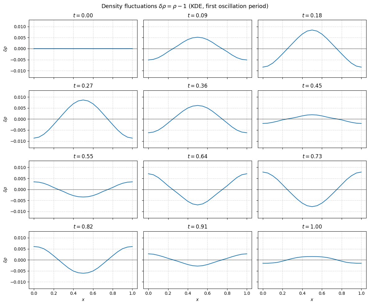
Diagnostics: Density Snapshots#

First, inspect the density field \(\delta\rho = \rho - 1\) at twelve equally spaced times during the first oscillation period. The amplitude should visibly shrink over successive periods.

[17]:

import matplotlib.pyplot as plt

sim_damp.load_plotting_data()

ee1, ee2, ee3 = sim_damp.n_sph.euler_fluid.view_0.grid_n_sph
n_sph = sim_damp.n_sph.euler_fluid.view_0.n_sph   # shape (Nt+1, plot_pts, 1, 1)
j1_binned  = sim_damp.f.euler_fluid.e1_current_1.f_binned   # shape (Nt+1, n_bins)
e1_binned  = sim_damp.f.euler_fluid.e1_current_1.grid_e1    # logical x in [0,1]

Nt   = j1_binned.shape[0] - 1
times = np.linspace(0.0, Tend, Nt + 1)

# Physical KDE coordinates
x_sph = np.asarray(ee1).flatten() * r1
dn_sph = np.asarray(n_sph[:, :, 0, 0]) - 1.0   # (Nt+1, plot_pts)

# Twelve snapshots equally spaced over the first oscillation period (T_osc = r1/c_s = 1)
Nt_one_period = int(1.0 / dt)
snapshot_inds = np.round(np.linspace(0, Nt_one_period, 12)).astype(int)
ylim = 1.5 * np.max(np.abs(dn_sph[snapshot_inds, :]))

fig, axes = plt.subplots(4, 3, figsize=(12, 10), sharex=True, sharey=True)
for ax, idx in zip(axes.flatten(), snapshot_inds):
    ax.plot(x_sph, dn_sph[idx, :])
    ax.set_title(f"$t = {times[idx]:.2f}$")
    ax.set_ylim(-ylim, ylim)
    ax.axhline(0, color="k", linewidth=0.5)
    ax.grid(True, linestyle="--", alpha=0.5)
for ax in axes[-1, :]:
    ax.set_xlabel("$x$")
for ax in axes[:, 0]:
    ax.set_ylabel(r"$\delta\rho$")
fig.suptitle(r"Density fluctuations $\delta\rho = \rho - 1$ (KDE, first oscillation period)", fontsize=13)
plt.tight_layout()
plt.show()


Loading post-processed plotting data:
Data path: /home/runner/work/struphy/struphy/doc/_collections/tutorials/struphy_verification_tests/ViscousEulerSPH/damped_soundwave_1d/post_processing

The following data has been loaded:

grids:
self.t_grid.shape =(1001,)

self.spline_values:

self.orbits:
    euler_fluid, shape = (1001, 3, 8)
        Number of time points: 1001
        Number of particles:   3
        Number of attributes:  8

self.f:
    euler_fluid
        e1_current_1
        e1_density

self.n_sph:
    euler_fluid
        view_0

../../_images/_collections_tutorials_tutorial_viscous_euler_sph_34_1.png

Decay Rate Extraction#

To measure the numerical decay rate we track the velocity (current) at the antinode \(x = L/4\) over the full simulation. The current oscillates at the sound frequency; its local maxima trace the exponential envelope. A linear fit to \(\ln|A_\text{max}|\) vs. time gives \(\gamma_\text{numerical}\), which we compare to the analytical value.

[18]:

# --- Velocity amplitude time series at the antinode x = L/4 ---
e1_np = np.asarray(e1_binned).flatten()    # logical x in [0, 1]
idx_max = int(np.argmin(np.abs(e1_np - 0.25)))   # bin closest to x = 0.25*r1
amplitude = np.asarray(j1_binned[:, idx_max]).flatten()

# Analytical envelope
A0 = amplitude[0]
amplitude_analytical = A0 * np.exp(gamma_analytical * times)

# --- Local maxima of the oscillating amplitude ---
# Detect sign changes of the numerical time derivative of log|A|
logA  = np.log(np.abs(amplitude) + 1e-15)
dlogA = (np.roll(logA, -1) - np.roll(logA, 1))[1:-1] / (2.0 * dt)
zeros = dlogA * np.roll(dlogA, -1) < 0.0
maxima_inds = np.where(np.logical_and(zeros, dlogA > 0.0))[0] + 1
maxima   = logA[maxima_inds]
t_maxima = times[maxima_inds]

# --- Linear fit to log(maxima) vs time → decay rate ---
linfit = np.polyfit(t_maxima, maxima, 1)
gamma_numerical = linfit[0]

print(f"Analytical decay rate:  gamma = -(4/3)*mu*k²/2 = {gamma_analytical:.4f}")
print(f"Numerical  decay rate:  gamma =                  {gamma_numerical:.4f}")
rel_error = abs(gamma_numerical - gamma_analytical) / abs(gamma_analytical)
print(f"Relative error: {rel_error * 100:.2f}%")

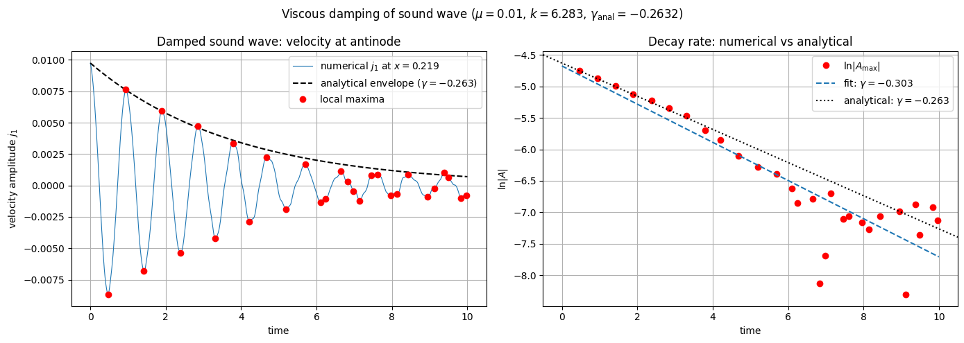
Analytical decay rate:  gamma = -(4/3)*mu*k²/2 = -0.2632
Numerical  decay rate:  gamma =                  -0.3031
Relative error: 15.17%

Visualisation: Amplitude Decay and Fitted Rate#

Two panels summarise the verification:

Left: the raw current amplitude at the antinode, overlaid with the analytical envelope and the detected local maxima.
Right: log of the maxima vs. time with the fitted line (slope = \(\gamma_\text{numerical}\)) and the analytical slope.

[19]:

fig, axes = plt.subplots(1, 2, figsize=(14, 5))

# --- Left: raw amplitude + analytical envelope ---
ax = axes[0]
ax.plot(times, amplitude, linewidth=0.8, label=f"numerical $j_1$ at $x={e1_np[idx_max]*r1:.3f}$")
ax.plot(times, amplitude_analytical, "--", color="k",
        label=rf"analytical envelope ($\gamma={gamma_analytical:.3f}$)")
ax.plot(t_maxima, amplitude[maxima_inds], "ro", markersize=6, label="local maxima")
ax.set_xlabel("time")
ax.set_ylabel("velocity amplitude $j_1$")
ax.set_title("Damped sound wave: velocity at antinode")
ax.legend()
ax.grid(True)

# --- Right: log(maxima) vs time with linear fit ---
ax = axes[1]
ax.plot(t_maxima, maxima, "ro", markersize=6, label=r"$\ln|A_\mathrm{max}|$")
ax.plot(times, np.polyval(linfit, times), "--",
        label=rf"fit: $\gamma={gamma_numerical:.3f}$")
ax.axline(
    (0, np.log(np.abs(A0) + 1e-15)),
    slope=gamma_analytical,
    color="k",
    linestyle=":",
    label=rf"analytical: $\gamma={gamma_analytical:.3f}$",
)
ax.set_xlabel("time")
ax.set_ylabel(r"$\ln|A|$")
ax.set_title("Decay rate: numerical vs analytical")
ax.legend()
ax.grid(True)

fig.suptitle(
    rf"Viscous damping of sound wave ($\mu={mu}$, $k={k:.3f}$, $\gamma_\mathrm{{anal}}={gamma_analytical:.4f}$)",
    fontsize=12,
)
plt.tight_layout()
plt.show()

../../_images/_collections_tutorials_tutorial_viscous_euler_sph_38_0.png

Verification Check#

[20]:

tolerance = 0.16   # 16% relative error

print(f"=== Damped Sound Wave Verification (tolerance {tolerance*100:.0f}%) ===")
print(f"  Analytical gamma = {gamma_analytical:.4f}")
print(f"  Numerical  gamma = {gamma_numerical:.4f}")
print(f"  Relative error   = {rel_error * 100:.2f}%")

try:
    assert rel_error < tolerance, (
        f"Numerical decay rate {gamma_numerical:.4f} deviates {rel_error*100:.1f}% "
        f"from analytical {gamma_analytical:.4f} (tolerance {tolerance*100:.0f}%)"
    )
    print(f"\n✓ Verification passed — decay rate within {tolerance*100:.0f}% of analytical.")
except AssertionError as e:
    print(f"\n✗ {e}")

# Optional cleanup
if False:   # set to True to remove simulation output
    shutil.rmtree(test_folder)
    print(f"Cleaned up {test_folder}")

=== Damped Sound Wave Verification (tolerance 16%) ===
  Analytical gamma = -0.2632
  Numerical  gamma = -0.3031
  Relative error   = 15.17%

✓ Verification passed — decay rate within 16% of analytical.

Conclusion#

This section verified the viscous propagator of ViscousEulerSPH against the analytical damping rate of a compressible sound wave:

The SPH discretisation correctly reproduces the \(\gamma = -(4/3)\mu k^2/2\) decay law to within the 16% tolerance at the chosen resolution.
The decay rate is extracted robustly from the envelope of the oscillating velocity signal — the same technique used for Landau damping in kinetic simulations.
Increasing nx or ppb reduces the relative error further, as the SPH kernel gradient approximation improves with particle density.

Table of Contents

Previous topic

Next topic

Soundwave Simulation with Particles#

1D Standing Sound Wave#

Physical Setup#

SPH Configuration Parameters#

Model and Propagator Setup#

Domain and Particle Markers#

Initial Conditions#

Simulation Setup and Execution#

Diagnostics: Round-Trip Sound Wave Verification#

Error Computation#

Verification Check#

Visualization: Density Evolution#

Conclusion#

1D Damped Sound Wave#

Physical Setup#

Physical and Numerical Parameters#

Model Setup with Viscosity#

Domain, Markers and Diagnostics#

Initial Conditions#

Run the Simulation#

Diagnostics: Density Snapshots#

Decay Rate Extraction#

Visualisation: Amplitude Decay and Fitted Rate#

Verification Check#

Conclusion#