FEEC#

Derham complex#

class struphy.feec.psydac_derham.DiscreteDerham(V0: TensorFemSpace, V1: VectorFemSpace, V2: VectorFemSpace, V3: TensorFemSpace)[source]#

Bases: object

Discrete 3D de Rham sequence built from four FE spaces.

Used internally by Derham (via Derham.init_derham) to create the base FE spaces and derivative operators before boundary, polar, and projector augmentations are added.

The sequence is represented as

V0 --grad--> V1 --curl--> V2 --div--> V3

where V0 is an H1-conforming scalar space, V1 an Hcurl vector space, V2 an Hdiv vector space, and V3 an L2 scalar space.

The auxiliary space (H^1)^3 for vector fields is also built for projection and polar extraction purposes, but it is not part of the proper de Rham sequence.

Moreover, the 1D FEM spaces (serial, not distributed) in each direction are built from the corresponding 3D spaces, and stored as attributes for building Kronecker matrices.

Parameters:

V0 (TensorFemSpace) – First space of the de Rham sequence : H1 space
V1 (VectorFemSpace) – Second space of the de Rham sequence : Hcurl space
V2 (VectorFemSpace) – Third space of the de Rham sequence : Hdiv space
V3 (TensorFemSpace) – Fourth space of the de Rham sequence : L2 space

Notes

On construction, differential operators are created and attached to the input spaces as convenience attributes:

V0.grad and V0.diff
V1.curl and V1.diff
V2.div and V2.diff

property dim: int#: Dimension of the physical and logical domains, which are assumed to be the same.

property V0: TensorFemSpace#

H1 space

Type:: First space of the de Rham sequence

property V1: VectorFemSpace#

Hcurl space

Type:: Second space of the de Rham sequence

property V2: VectorFemSpace#

Hdiv space

Type:: Third space of the de Rham sequence

property V3: TensorFemSpace#

L2 space

Type:: Fourth space of the de Rham sequence

property Vv: VectorFemSpace#: Auxiliary H1^3 space for vector fields, used for projection and polar extraction purposes.

property spaces: tuple[TensorFemSpace | VectorFemSpace, ...]#: Spaces of the proper de Rham sequence (excluding Hvec).

property derivatives_as_matrices#: Differential operators of the De Rham sequence as LinearOperator objects.

property derivatives#

Differential operators of the De Rham sequence as DiffOperator objects.

Those are objects with domain and codomain properties that are FemSpace, they act on FemField (they take a FemField of their domain as input and return a FemField of their codomain.

property H1_1d_serial: tuple[TensorFemSpace, TensorFemSpace, TensorFemSpace]#: The 1D H1 spaces in each direction (no domain decomposition), built from the corresponding 3D spaces.

property L2_1d_serial: tuple[TensorFemSpace, TensorFemSpace, TensorFemSpace]#: The 1D L2 spaces in each direction (no domain decomposition), built from the corresponding 3D spaces.

projectors(*, kind='global', nquads=None) → tuple[GlobalGeometricProjector, ...][source]#

Projectors mapping callable functions of the physical coordinates to a corresponding FemField object in the De Rham sequence.

Parameters:

kind (str) – Type of the projection : at the moment, only global is accepted and returns geometric commuting projectors based on interpolation/histopolation for the De Rham sequence (GlobalGeometricProjector objects).
nquads (list(int) | tuple(int)) – Number of quadrature points along each direction, to be used in Gauss quadrature rule for computing the (approximated) degrees of freedom.

Returns:

P0, …, Pn – Projectors that can be called on any callable function that maps from the physical space to R (scalar case) or R^d (vector case) and returns a FemField belonging to the i-th space of the De Rham sequence

Return type:

callables

__weakref__#: list of weak references to the object (if defined)

class struphy.feec.psydac_derham.SplineAttributes1D(femspace: TensorFemSpace | VectorFemSpace, nquads: tuple[int, int, int], nquads_proj: tuple[int, int, int], polar_splines: bool = False, local_projectors: bool = False)[source]#

Bases: object

Container for 1D spline metadata extracted from a 3D FE space.

This helper precomputes and stores per-direction information needed by projection operators, quadrature-based assembly, and spline evaluation kernels. It supports both scalar (TensorFemSpace) and vector-valued (VectorFemSpace) spaces.

Parameters:

femspace (TensorFemSpace | VectorFemSpace) – Finite-element space from which the 1D spline information is derived.
nquads (tuple[int, int, int]) – Number of quadrature points in each logical direction (eta_1, eta_2, eta_3) for numerical integration grids.
nquads_proj (tuple[int, int, int]) – Number of quadrature points in each logical direction used to build projection point/weight sets.
polar_splines (bool, default=False) – Polar spline regularity flag. False selects standard tensor-product splines, while True enables C1 polar splines (including the optional shift of points near eta_1 = 0 where required).
local_projectors (bool, default=False) – If True, also computes quasi-interpolation point/weight grids used by local commuting projectors.

Notes

Data layout depends on the input space type:

scalar space: each attribute is indexed by direction;
vector space: each attribute is indexed by component, then direction.

The class stores:

spline descriptors (number of basis functions, spline kind),
projection grids (points, weights, sub-interval markers),
optional local-projector grids,
quadrature grids (points, weights, spans, basis values).

property femspace: TensorFemSpace | VectorFemSpace#: The 3d tensor product spline space (scalar or vector valued) from which the 1d spline space information is derived.

property nquads: tuple[int, int, int]#: The number of quadrature points in each direction for numerical integration.

property nquads_proj: tuple[int, int, int]#: The number of quadrature points in each direction for the projection.

property polar_splines: bool#: The polar splines flag.

property local_projectors: bool#: Whether to use local projectors.

property tensor_spaces: tuple[TensorFemSpace, ...]#: The underlying tensor product spaces (one per component for vector-valued spaces).

property nbasis: tuple[tuple[int]]#: Tuple of number of basis functions in each direction for each component of the vector space.

property spline_types: tuple[tuple[str]]#: Tuple of spline types in each direction (‘B’ or ‘M’) for each component of the vector space.

property spline_types_pyccel: tuple[ndarray]#: Tuple of spline types in each direction as integers (0 for ‘B’, 1 for ‘M’) for each component of the vector space.

property proj_grid_pts: tuple[tuple[ndarray]]#: Tuple of projection grid points in each direction for each component of the vector space.

property proj_grid_wts: tuple[tuple[ndarray]]#: Tuple of projection grid weights in each direction for each component of the vector space.

property proj_grid_subs: tuple[tuple[ndarray]]#: Tuple of projection grid sub-interval indices in each direction for each component of the vector space.

property proj_loc_grid_pts: tuple[tuple[ndarray]] | None#: Tuple of local projection grid points in each direction for each component of the vector space.

property proj_loc_grid_wts: tuple[tuple[ndarray]] | None#: Tuple of local projection grid weights in each direction for each component of the vector space.

property quad_grid_pts: tuple[tuple[ndarray]]#: Tuple of quadrature grid points in each direction for each component of the vector space.

property quad_grid_wts: tuple[tuple[ndarray]]#: Tuple of quadrature grid weights in each direction for each component of the vector space.

property quad_grid_spans: tuple[tuple[ndarray]]#: Tuple of quadrature grid basis function spans in each direction for each component of the vector space.

property quad_grid_bases: tuple[tuple[ndarray]]#: Tuple of quadrature grid basis function values in each direction for each component of the vector space.

__weakref__#: list of weak references to the object (if defined)

class struphy.feec.psydac_derham.Derham(grid: TensorProductGrid, options: DerhamOptions, comm: Intracomm | None = None, domain: Domain | None = None)[source]#

Bases: object

High-level discrete de Rham complex on the 3D logical unit cube.

The class builds a tensor-product base complex through DiscreteDerham and augments it with optional boundary enforcement, optional C1 polar extraction operators, and commuting projectors. It also stores convenient metadata (1D spline attributes, decomposition helpers, index arrays) used by initialization, evaluation, and kernel interfaces.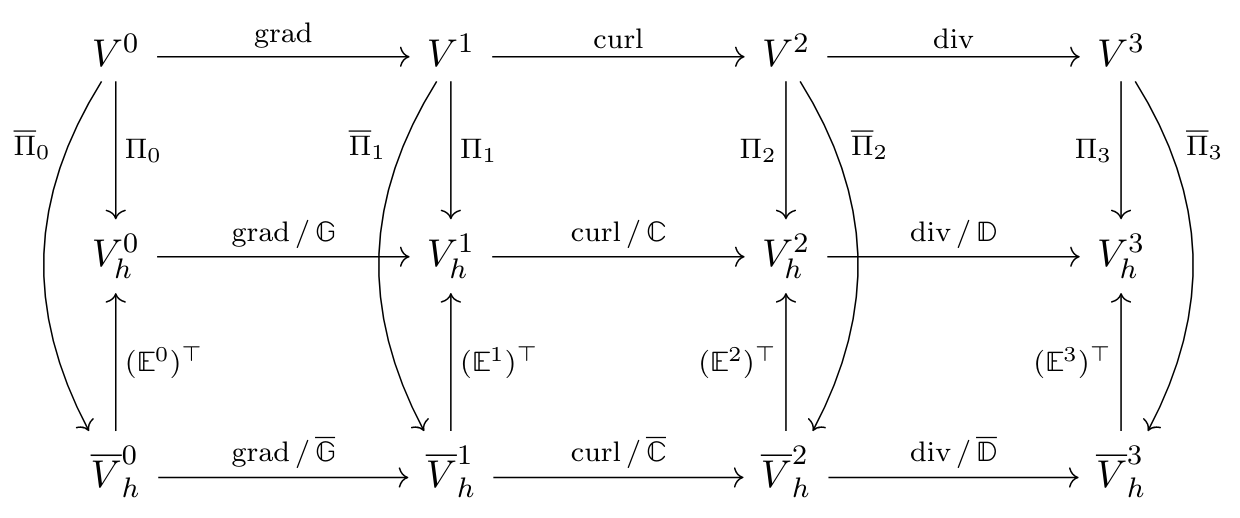

Parameters:

grid (TensorProductGrid) – The FEEC grid.
options (DerhamOptions) – The options for building the discrete de Rham sequence, including spline degrees, boundary conditions, quadrature options, polar spline options, and projector options.
comm (Intracomm) – MPI communicator (sub_comm if clones are used).
domain (Domain, optional) – The Struphy domain object for evaluating the mapping F : [0, 1]^3 –> R^3 and the corresponding metric coefficients.

Notes

The underlying base sequence is

V0 --grad--> V1 --curl--> V2 --div--> V3.

An auxiliary H1vec FEM space is also built for vector-field projection and polar extraction machinery.

property grid: TensorProductGrid#: The FEEC grid.

property options: DerhamOptions#: The DerhamOptions object containing the input options for the Derham sequence construction.

property comm#: MPI communicator.

property domain: Domain | None#: Mapping from logical unit cube to physical domain (only needed in case of polar splines with polar_splines is True).

property num_elements: tuple[int, int, int]#: List of number of elements (=cells) in each direction.

property degree: tuple[int, int, int]#: List of B-spline degrees in each direction.

property bcs: tuple[None | tuple[Literal['free', 'dirichlet'], Literal['free', 'dirichlet']], None | tuple[Literal['free', 'dirichlet'], Literal['free', 'dirichlet']], None | tuple[Literal['free', 'dirichlet'], Literal['free', 'dirichlet']]]#: Tuple of boundary conditions in each direction. Each entry is either None (periodic) or a tuple with two entries (left and right boundary), “dirichlet” or “free” (clamped splines).

property nquads: tuple[int, int, int]#: List of number of Gauss-Legendre quadrature points in each direction (default = degree, leads to exact integration of degree 2p-1 polynomials).

property nquads_proj: tuple[int, int, int]#: List of number of Gauss-Legendre quadrature points in histopolation (default = degree + 1) in each direction.

property mpi_dims_mask: tuple[bool, bool, bool]#: List of bool indicating which dimensions are decomposed in the MPI domain decomposition.

property with_projectors: bool#: True if global commuting projectors are to be assembled.

property polar_splines: bool#: C^k smoothness at eta_1=0. Is False for standard tensor product splines and True for C^1 polar splines.

property with_local_projectors: bool#: True if local projectors are to be used instead of the default global ones.

property V0fem: TensorFemSpace#: Psydac’s finite element space for 0-forms (scalar H1).

property V1fem: VectorFemSpace#: Psydac’s finite element space for 1-forms (vector Hcurl).

property V2fem: VectorFemSpace#: Psydac’s finite element space for 2-forms (vector Hdiv).

property V3fem: TensorFemSpace#: Psydac’s finite element space for 3-forms (scalar L2).

property Vvfem: VectorFemSpace#: Psydac’s finite element space for vector H1 fields (not part of the proper de Rham sequence, but useful for the projectors and polar extraction operators).

property H1_1d_serial: tuple[SplineSpace, SplineSpace, SplineSpace]#: Tuple of 1D H1 spline spaces in each direction (no domain decomposition).

property L2_1d_serial: tuple[SplineSpace, SplineSpace, SplineSpace]#: Tuple of 1D L2 spline spaces in each direction (no domain decomposition).

property fem_spaces: dict[str, TensorFemSpace | VectorFemSpace]#: Dictionary mapping form names to their corresponding finite element spaces.

property V0splines: SplineAttributes1D#: 1D spline attributes for the 0-form space (scalar H1).

property V1splines: SplineAttributes1D#: 1D spline attributes for the 1-form space (vector Hcurl).

property V2splines: SplineAttributes1D#: 1D spline attributes for the 2-form space (vector Hdiv).

property V3splines: SplineAttributes1D#: 1D spline attributes for the 3-form space (scalar L2).

property Vvsplines: SplineAttributes1D#: 1D spline attributes for the H1^3 space (not part of the proper de Rham sequence, but useful for the projectors and polar extraction operators).

property H1_1d_serial_splines: tuple[SplineAttributes1D]#: Tuple of 1D spline attributes for the H1_1d_serial spaces in each direction.

property L2_1d_serial_splines: tuple[SplineAttributes1D]#: Tuple of 1D spline attributes for the L2_1d_serial spaces in each direction.

property spline_attributes: dict[str, SplineAttributes1D]#: Dictionary mapping form names to their corresponding 1D spline attributes.

property V0: StencilVectorSpace#: Coefficient space for 0-forms (scalar H1).

property V1: BlockVectorSpace#: Coefficient space for 1-forms (vector Hcurl).

property V2: BlockVectorSpace#: Coefficient space for 2-forms (vector Hdiv).

property V3: StencilVectorSpace#: Coefficient space for 3-forms (scalar L2).

property Vv: BlockVectorSpace#: Coefficient space for vector fields in H1^3 (not part of the proper de Rham sequence, but useful for the projectors and polar extraction operators).

property coeff_spaces: dict[str, StencilVectorSpace | BlockVectorSpace]#: Dictionary mapping form names to their corresponding coefficient spaces.

property V0pol: StencilVectorSpace | PolarDerhamSpace#: Coefficient space for 0-forms (scalar H1) for polar splines.

property V1pol: BlockVectorSpace | PolarDerhamSpace#: Coefficient space for 1-forms (vector Hcurl) for polar splines.

property V2pol: BlockVectorSpace | PolarDerhamSpace#: Coefficient space for 2-forms (vector Hdiv) for polar splines.

property V3pol: StencilVectorSpace | PolarDerhamSpace#: Coefficient space for 3-forms (scalar L2) for polar splines.

property Vvpol: BlockVectorSpace | PolarDerhamSpace#: Coefficient space for vector fields in H1^3 for polar splines (not part of the proper de Rham sequence, but useful for the projectors and polar extraction operators).

property polar_coeff_spaces: dict[str, StencilVectorSpace | BlockVectorSpace | PolarDerhamSpace]#: Dictionary mapping form names to their corresponding coefficient spaces for polar splines.

property ck_blocks: PolarExtractionBlocksC1 | None#: Polar extraction blocks for C1 polar splines. Is None if polar_splines is False (standard tensor product splines).

property space_to_form: dict[str, str]#: Dictionary mapping space names to form names. The form names are “0”, “1”, “2”, “3” for the proper de Rham sequence, and “v” for the H1^3 space.

property grad#: Discrete gradient H1 -> Hcurl.

property curl#: Discrete curl Hcurl -> Hdiv.

property div#: Discrete divergence Hdiv -> L2.

property P0: CommutingProjector | CommutingProjectorLocal#: Commuting projector to 0-forms (interpolation). If self.with_local_projectors is True, the local projector is chosen.

property P1: CommutingProjector | CommutingProjectorLocal#: Commuting projector to 1-forms (interpolation and histopolation). If self.with_local_projectors is True, the local projector is chosen.

property P2: CommutingProjector | CommutingProjectorLocal#: Commuting projector to 2-forms (interpolation and histopolation). If self.with_local_projectors is True, the local projector is chosen.

property P3: CommutingProjector | CommutingProjectorLocal#: Commuting projector to 3-forms (histopolation). If self.with_local_projectors is True, the local projector is chosen.

property Pv: CommutingProjector | CommutingProjectorLocal#: Commuting projector to H1^3 space (interpolation). If self.with_local_projectors is True, the local projector is chosen.

property projectors: dict[str, CommutingProjector | CommutingProjectorLocal]#: Dictionary mapping form names to their corresponding projectors. The form names are “0”, “1”, “2”, “3” for the proper de Rham sequence, and “v” for the H1^3 space.

property P0glob#: Global version of the commuting projector to 0-forms (interpolation). Only available if self.with_local_projectors is True.

property P1glob#: Global version of the commuting projector to 1-forms (interpolation and histopolation). Only available if self.with_local_projectors is True.

property P2glob#: Global version of the commuting projector to 2-forms (interpolation and histopolation). Only available if self.with_local_projectors is True.

property P3glob#: Global version of the commuting projector to 3-forms (histopolation). Only available if self.with_local_projectors is True.

property Pvglob#: Global version of the commuting projector to H1^3 space (interpolation). Only available if self.with_local_projectors is True.

property projectors_global#: Dictionary mapping form names to their corresponding global projectors. The form names are “0”, “1”, “2”, “3” for the proper de Rham sequence, and “v” for the H1^3 space. Only available if self.with_local_projectors is True.

property P0loc#: Local version of the commuting projector to 0-forms (interpolation). Only available if self.with_local_projectors is True.

property P1loc#: Local version of the commuting projector to 1-forms (interpolation and histopolation). Only available if self.with_local_projectors is True.

property P2loc#: Local version of the commuting projector to 2-forms (interpolation and histopolation). Only available if self.with_local_projectors is True.

property P3loc#: Local version of the commuting projector to 3-forms (histopolation). Only available if self.with_local_projectors is True.

property Pvloc#: Local version of the commuting projector to H1^3 space (interpolation). Only available if self.with_local_projectors is True.

property projectors_local#: Dictionary mapping form names to their corresponding local projectors. The form names are “0”, “1”, “2”, “3” for the proper de Rham sequence, and “v” for the H1^3 space. Only available if self.with_local_projectors is True.

property spl_kind: tuple[bool]#: Tuple of bool indicating the kind of spline in each direction (True=periodic, False=clamped).

property dirichlet_bc: tuple[tuple[bool, bool]]#: Tuple of tuples indicating whether homogeneous Dirichlet boundary conditions are applied at left and right boundary in each direction.

property breaks#: List of break points (=cell interfaces) in each direction.

property indN#: List of 2d arrays holding global spline indices (N) in each element in the three directions.

property indD#: List of 2d arrays holding global spline indices (D) in each element in the three directions.

property domain_decomposition#: Psydac’s domain decomposition object (same for all vector spaces!).

property domain_array#

A 2d array[float] of shape (comm.Get_size(), 9). The row index denotes the process number and for n=0,1,2:

domain_array[i, 3*n + 0] holds the LEFT domain boundary of process i in direction eta_(n+1).

domain_array[i, 3*n + 1] holds the RIGHT domain boundary of process i in direction eta_(n+1).

domain_array[i, 3*n + 2] holds the number of cells of process i in direction eta_(n+1).

property breaks_loc#: The domain local to this process.

property index_array#

A 2d array[int] of shape (comm.Get_size(), 6). The row index denotes the process number and for n=0,1,2:

arr[i, 2*n + 0] holds the global start index of cells of process i in direction eta_(n+1).

arr[i, 2*n + 1] holds the global end index of cells of process i in direction eta_(n+1).

property index_array_N#

A 2d array[int] of shape (comm.Get_size(), 6). The row index denotes the process number and for n=0,1,2:

arr[i, 2*n + 0] holds the global start index of B-splines (N) of process i in direction eta_(n+1).

arr[i, 2*n + 1] holds the global end index of B-splines (N) of process i in direction eta_(n+1).

property index_array_D#

A 2d array[int] of shape (comm.Get_size(), 6). The row index denotes the process number and for n=0,1,2:

arr[i, 2*n + 0] holds the global start index of M-splines (D) of process i in direction eta_(n+1).

arr[i, 2*n + 1] holds the global end index of M-splines (D) of process i in direction eta_(n+1).

property neighbours#: A 3d array[int] with shape (3,3,3). It contains the 26 neighbouring process ids (rank). This is done in terms of N-spline start/end indices. The i-th index indicates direction eta_(i+1). 0 is a left neighbour, 1 is the same plane as the current process, 2 is a right neighbour. For more detail see _get_neighbours().

property extraction_ops#: Dictionary holding basis extraction operators, either IdentityOperator or PolarExtractionOperator.

property dofs_extraction_ops#: Dictionary holding dof extraction operators for commuting projectors, either IdentityOperator or PolarExtractionOperator.

property boundary_ops#: Dictionary holding essential boundary operators (BoundaryOperator) OR IdentityOperators.

property grad_bcfree#: Discrete gradient Vh0_pol (H1) -> Vh1_pol (Hcurl) w/o boundary operator.

property curl_bcfree#: Discrete curl Vh1_pol (Hcurl) -> Vh2_pol (Hdiv) w/o boundary operator.

property div_bcfree#: Discrete divergence Vh2_pol (Hdiv) -> Vh3_pol (L2) w/o boundary operator.

property args_derham#: Collection of mandatory arguments for pusher kernels.

to_dict() → dict[source]#: Serialize the Derham configuration to a dictionary. The MPI communicator is not serialized and set to None.

classmethod from_dict(dct, comm: Intracomm | None = None) → Derham[source]#: Deserialize a Derham configuration from a dictionary. The MPI communicator is set to None.

init_derham(num_elements: tuple[int, int, int], degree: tuple[int, int, int], spl_kind: tuple[bool, bool, bool], comm=None, mpi_dims_mask: tuple[bool, bool, bool] | None = None, use_feectools: bool = True) → DiscreteDerham[source]#

Return a discrete Derham complex. Allows for the use of tiny-feectools.

Parameters:

num_elements (tuple[int, int, int]) – Number of elements in each direction.
degree (tuple[int, int, int]) – Spline degree in each direction.
spl_kind (tuple[bool, bool, bool]) – Kind of spline in each direction (True=periodic, False=clamped).
comm (mpi4py.MPI.Intracomm) – MPI communicator (within a clone if domain cloning is used, otherwise MPI.COMM_WORLD)
mpi_dims_mask (tuple[bool, bool, bool]) – True if the dimension is to be used in the domain decomposition (=default for each dimension). If mpi_dims_mask[i]=False, the i-th dimension will not be decomposed.
use_feectools (bool) – Use slimmed-down fork feectools of Psydac.

Creat a callable spline function.

Parameters:

name (str) – Field’s key to be used for instance when saving to hdf5 file.
space_id (str) – Space identifier for the field (“H1”, “Hcurl”, “Hdiv”, “L2” or “H1vec”).
coeffs (StencilVector | BlockVector) – The spline coefficients.
backgrounds (FieldsBackground | list) – For the initial condition.
perturbations (Perturbation | list) – For the initial condition.
domain (Domain) – Mapping for pullback/transform of initial condition.
equil (FLuidEquilibrium) – Fluid background used for inital condition.

prepare_eval_tp_fixed(grids_1d)[source]#

Obtain knot span indices and spline basis functions evaluated at tensor product grid.

Parameters:

grids_1d (3-list of 1d arrays) – Points of the tensor product grid.

Returns:

spans (3-tuple of 2d int arrays) – Knot span indices in each direction in format (n, nq).
bns (3-tuple of 3d float arrays) – Values of degree + 1 non-zero B-Splines at quadrature points in format (n, nq, basis).
bds (3-tuple of 3d float arrays) – Values of degree non-zero D-Splines at quadrature points in format (n, nq, basis).

__weakref__#: list of weak references to the object (if defined)

Bases: object

Initializes a callable spline function with a method for assigning initial conditions.

Parameters:

name (str) – Field’s key to be used for instance when saving to hdf5 file.
space_id (str) – Space identifier for the field (“H1”, “Hcurl”, “Hdiv”, “L2” or “H1vec”).
derham (struphy.feec.psydac_derham.Derham) – Discrete Derham complex.
coeffs (StencilVector | BlockVector) – The spline coefficients (optional).
backgrounds (FieldsBackground | list) – For the initial condition.
perturbations (Perturbation | list) – For the initial condition.
domain (Domain) – Mapping for pullback/transform of initial condition.
equil (FluidEquilibrium) – Fluid background used for inital condition.

__weakref__#: list of weak references to the object (if defined)

property name#: Name of the field in data container (string).

property space_id#

‘H1’, ‘Hcurl’, ‘Hdiv’, ‘L2’ or ‘H1vec’.

Type:: String identifying the continuous space of the field

property space_key#

‘0’, ‘1’, ‘2’, ‘3’ or ‘v’.

Type:: String identifying the discrete space of the field

property derham#: 3d Derham complex struphy.feec.psydac_derham.Derham.

property domain#: Mapping for pullback/transform of initial condition.

property equil#: Fluid equilibirum used for initial condition.

property space#: Coefficient space (VectorSpace) of the field.

property fem_space#: FE space (FemSpace) of the field.

property ET#: Transposed PolarExtractionOperator (or IdentityOperator) for mapping polar coeffs to polar tensor product rings.

property vector#: feectools.linalg.stencil.StencilVector or feectools.linalg.block.BlockVector or struphy.polar.basic.PolarVector.

property starts#: Global indices of the first FE coefficient on the process, in each direction.

property ends#: Global indices of the last FE coefficient on the process, in each direction.

property pads#: Paddings for ghost regions, in each direction.

property nbasis#: Tuple(s) of 1d dimensions for each direction.

property vector_stencil#

Tensor-product Stencil-/BlockVector corresponding to a copy of self.vector in case of Stencil-/Blockvector

OR

the extracted coefficients in case of PolarVector. Call self.extract_coeffs() beforehand.

property backgrounds: FieldsBackground | list#: For the initial condition.

property perturbations: Perturbation | list#: For the initial condition.

extract_coeffs(update_ghost_regions=True)[source]#

Maps polar coeffs to polar tensor product rings in case of PolarVector (written in-place to self.vector_stencil) and updates ghost regions.

Parameters:: update_ghost_regions (bool) – If the ghost regions shall be updated (needed in case of non-local acccess, e.g. in field evaluation).

initialize_coeffs(*, backgrounds: FieldsBackground | list | None = None, perturbations: Perturbation | list | None = None, domain: Domain | None = None, equil: FluidEquilibrium | None = None)[source]#: Set the initial conditions for self.vector.

initialize_coeffs_from_restart_file(file, key)[source]#: TODO

eval_tp_fixed_loc(spans, bases, out=None)[source]#

Spline evaluation on pre-defined grid.

Input spans must be on local process, start <= span <= end.

Parameters:

spans (3-tuple of 1d int arrays) – Knot span indices in each direction (start <= span <= end).
bases (3-tuple of 2d float arrays) – Values of non-zero eta basis functions at evaluation points indexed by (eta, basis function).

Returns:

out – 3d array of spline values S_ijk corresponding to the sizes of spans.

Return type:

array[float]

__call__(*etas, out=None, tmp=None, squeeze_out=False, local=False)[source]#

Evaluates the spline function on the global domain, unless local=True, in which case the spline function is evaluated only on the local domain, and the rest is set to zero.

Parameters:

*etas (array-like | tuple)
possible (Logical coordinates at which to evaluate. Two cases are) –
1. 2d numpy array, where coordinates are taken from eta1 = etas[:, 0], eta2 = etas[:, 1], etc. (like markers).
2. list/tuple (eta1, eta2, …), where eta1, eta2, … can be float or array-like of various shapes.
out (array[float] or list) – Array in which to store the values of the spline function at the given point set (list in case of vector-valued spaces).
tmp (array[float]) – Array that has shape the size of the grid that will be used as a temporary for AllReduce, to avoid creating it a each call.
flat_eval (bool) – Whether to do a flat evaluation, i.e. f([e11, e12], [e21, e22]) = [f(e11, e21), f(e12, e22)].
squeeze_out (bool) – Whether to remove singleton dimensions in output “values”.

Returns:

out – The values of the spline function at the given point set (list in case of vector-valued spaces).

Return type:

array[float] or list

copy()[source]#: Returns a shallow copy of the SplineFunction instance, but with a new coeffs vector.

struphy.feec.psydac_derham.transform_perturbation(pert_type: str, pert_params: dict, space_key: str, domain: Domain)[source]#

Creates callabe(s) from perturbation parameters.

Parameters:

pert_type (str) – Class name of the perturbation, see perturbations.
pert_params (dict) – Parameters of the perturbation.
space_key (str) – The p-form representation of the output: ‘0’, ‘1’, ‘2’ ‘3’ or ‘v’.
domain (Domain) – Domain object (mapping).

Returns:

fun – A callable or list of callables in the space defined by space_key.

Return type:

list

struphy.feec.psydac_derham.get_pts_and_wts(space_1d, start, end, n_quad=None, polar_shift=False)[source]#

Obtain local (to MPI process) projection point sets and weights in one grid direction.

Parameters:

space_1d (SplineSpace) – Psydac object for uni-variate spline space.
start (int) – Start index on current process.
end (int) – End index on current process.
n_quad (int) – Number of quadrature points for Gauss-Legendre histopolation. If None, is set to degree + 1 where degree is the space_1d degree (products of basis functions are integrated exactly).
polar_shift (bool) – Whether to shift the first interpolation point away from 0.0 by 1e-5 (needed only in eta_1 and for polar domains).

Returns:

pts (2D float array) – Quadrature points (or Greville points for interpolation) in format (ii, iq) = (interval, quadrature point).
wts (2D float array) – Quadrature weights (or 1’s for interpolation) in format (ii, iq) = (interval, quadrature point).
subs (1D int array) – One entry for each interval ii; usually has value 0. A value of 1 indicates that the cell ii is the second subinterval of a split Greville cell (for histopolation with even degree).

struphy.feec.psydac_derham.get_pts_and_wts_quasi(space_1d: SplineSpace, *, polar_shift: bool = False) → tuple[ndarray, ndarray][source]#

Obtain local projection point sets and weights in one grid direction for the quasi-interpolation method. The quasi-interpolation points are \(\nu - \mu +p\) equidistant points \(\{ x^i_j \}_{0 \leq j < \nu - \mu +p}\) in the sub-interval \(Q = [\eta_\mu , \eta_\nu]\) given by:

begin{itemize}

item Clamped: .. math:

Q = \left\{\begin{array}{lr}
[\eta_p = 0, \eta_{p+1}], & i = 0 \,,\\
{[\eta_p = 0, \eta_{p+i}]}, & 0 < i < p-1\,,\\
{[\eta_{i+1}, \eta_{i+p}]}, & p-1 \leq i \leq \hat{n}_N - p\,,\\
{[\eta_{i+1}, \eta_{\hat{n}_N} = 1]}, &  \hat{n}_N - p < i < \hat{n}_N -1\,,\\
{[\eta_{\hat{n}_N -1}, \eta_{\hat{n}_N} = 1]}, & i = \hat{n}_N -1 \,.
\end{array} \; \right .

item Periodic: .. math:

Q = [\eta_{i + 1}, \eta_{i + p}] \:\:\:\:\: \forall \:\: i.

end{itemize}

Which are allways a subset of \(\{-(p-1)h,-(p-1)h + \frac{h}{2}, ..., 1-h - \frac{h}{2},1-h \}\) for the periodic case.

Parameters:

space_1d (SplineSpace) – Psydac object for uni-variate spline space.
polar_shift (bool) – Whether to shift the first interpolation point away from 0.0 by 1e-5 (needed only in eta_1 and for polar domains).

Returns:

pts (2D float array) – Quadrature points (or quasi-interpolation points for interpolation) in format (ii, iq) = (interval, quadrature point).
wts (2D float array) – Quadrature weights (or 1’s for interpolation) in format (ii, iq) = (interval, quadrature point).

struphy.feec.psydac_derham.get_span_and_basis(pts, space)[source]#

Compute the knot span index and the values of degree + 1 basis function at each point in pts.

Parameters:

pts (xp.array) – 2d array of points (ii, iq) = (interval, quadrature point).
space (SplineSpace) – Psydac object, the 1d spline space to be projected.

Returns:

span (xp.array) – 2d array indexed by (n, nq), where n is the interval and nq is the quadrature point in the interval.
basis (xp.array) – 3d array of values of basis functions indexed by (n, nq, basis function).

struphy.feec.psydac_derham.get_weights_local_projector(pts, fem_space)[source]#

Compute the geometric weights for interpolation and histopolation. Should be called only with the grid points for 0-forms.

Parameters:

pts (xp.array) – 3d array of points. Contains the quasi-interpolation points in each direction.
fem_space (SplineSpace) – Psydac object, the 1d spline space to be projected. Should be the 0-form space.

Returns:

wij (List of xp.array) – List of 2d array indexed by (space_direction, i, j), where i determines for which FEEC coefficient this weights are needed. Used for interpolation.
whij (List of xp.array) – List of 2d array indexed by (space_direction, i, j), where i determines for which FEEC coefficient this weights are needed. Used for histopolation.

struphy.feec.psydac_derham.select_basis_local(i, degree, Nbasis, periodic)[source]#

Determines the start and end indices of the basis functions that must be taken from the collocation matrix to compute the geometric weights wij, for any given i.

Parameters:

i (int) – Index of the wij weights that must be computed.
degree (int) – B-spline degree.
Nbasis (int) – Number of B-spline.
periodic (bool) – Whether we have periodic boundary conditions.

Returns:

start (int) – Start index of the B-splines that must be consider in the collocation matrix to obtain the wij weights. Inclusive index
end (int) – End index of the B-splines that must be consider in the collocation matrix to obtain the wij weights. Exclusive index

Grids#

class struphy.topology.grids.TensorProductGrid(num_elements: Tuple[int, int, int] = (24, 10, 1), mpi_dims_mask: Tuple[bool, bool, bool] = (True, True, True))[source]#

Bases: OptionsBase

Grid as a tensor product of 1d grids.

Parameters:

num_elements (Tuple[int, int, int]) – Number of elements in each direction.
mpi_dims_mask (Tuple[bool, bool, bool]) – True if the dimension is to be used in the domain decomposition (=default for each dimension). If mpi_dims_mask[i]=False, the i-th dimension will not be decomposed.

__eq__(other)#: Return self==value.

__hash__ = None#

Mass Operators (bilinear forms)#

class struphy.feec.mass.WeightedMassOperators(derham: Derham, domain: Domain, eq_mhd: MHDequilibrium | None = None, matrix_free: bool = False)[source]#

Bases: object

Collection of pre-defined struphy.feec.mass.WeightedMassOperator.

Parameters:

derham (Derham) – Discrete de Rham sequence on the logical unit cube.
domain (Geometry) – Mapping from logical unit cube to physical domain and corresponding metric coefficients.
eq_mhd (MHDequilibrium | None) – MHD equilibrium object.
matrix_free (bool) – If set to true will not compute the matrix associated with the operator but directly compute the product when called.

property derham: Derham#: Discrete de Rham sequence on the logical unit cube.

property domain: Domain#: Mapping from the logical unit cube to the physical domain with corresponding metric coefficients.

property eq_mhd: MHDequilibrium | None#: MHD equilibrium object.

property matrix_free: bool#: If set to true will not compute the matrix associated with the operators but directly compute the dot product when called.

property M0#

𝕄⁰ijk, mno = ∫ Λ⁰ᵢⱼₖ Λ⁰ₘₙₒ √g dη.

Type:: Standard mass matrix for 0-forms (H1 space)

property M1#

𝕄¹(μ,ijk), (ν,mno) = ∫ Λ→¹μ,ijk G⁻¹ Λ→¹ν, mno √g dη.

Type:: Standard mass matrix for 1-forms (Hcurl space) as 3x3 block matrix indexed by <code>(μ, ν)</code>

property M2#

𝕄²(μ,ijk), (ν,mno) = ∫ Λ→²μ,ijk G Λ→²ν, mno 1√g dη.

Type:: Standard mass matrix for 2-forms (Hdiv space) as 3x3 block matrix indexed by <code>(μ, ν)</code>

property M3#

𝕄³ijk, mno = ∫ Λ³ᵢⱼₖ Λ³ₘₙₒ 1√g dη.

Type:: Standard mass matrix for 3-forms (L2 space)

property Mv#

𝕄ᵛ(μ,ijk), (ν,mno) = ∫ Λ→ᵛμ,ijk G Λ→ᵛν, mno √g dη.

Type:: Standard mass matrix for vector 0-forms (H1vec space) as 3x3 block matrix indexed by <code>(μ, ν)</code>

property M2stab_for_rot#

𝕄²(μ,ijk), (ν,mno) = ∫ Λ→²μ,ijk Λ→²ν, mno 1√g dη.

Type:: Stabilization matrix for the rot-problem u2 + B2 x u2 = G*f2 as 3x3 block matrix indexed by <code>(μ, ν)</code>

property M1n#

Mass matrix

𝕄1,n(μ,ijk), (ν,mno) = ∫ n⁰eq(η) Λ→¹μ,ijk G⁻¹ Λ→¹ν,mno √g dη.

where <code>n⁰eq(η)</code> is an MHD equilibrium density (0-form).

property M2n#

Mass matrix

𝕄2,n(μ,ijk), (ν,mno) = ∫ n⁰eq(η) Λ→²μ,ijk G Λ→²ν,mno 1√g dη.

where <code>n⁰eq(η)</code> is an MHD equilibrium density (0-form).

property Mvn#

Mass matrix

𝕄v,n(μ,ijk), (ν,mno) = ∫ n⁰eq(η) Λ→ᵛμ,ijk G Λ→ᵛν,mno √g dη.

where <code>n⁰eq(η)</code> is an MHD equilibrium density (0-form).

property M1ninv#

Mass matrix

𝕄1,1n(μ,ijk), (ν,mno) = ∫ 1n⁰eq(η) Λ→¹μ,ijk G⁻¹ Λ→¹ν,mno √g dη.

where <code>n⁰eq(η)</code> is an MHD equilibrium density (0-form).

property M1J#

Mass matrix

𝕄1,J(μ,ijk), (ν,mno) = ∫ Λ→¹μ,ijk G⁻¹ ℛ(J) Λ→²ν,mno dη.

with the rotation matrix

ℛ(J)α,ν := εαβν J²eq,β, s.t. ℛ(J) v→ = J→²eq × v→,

where <code>εα β ν</code> stands for the Levi-Civita tensor and <code>J²eq, β</code> is the <code>β</code>-component of the MHD equilibrium current density (2-form).

property M2J#

Mass matrix

𝕄2,J(μ,ijk), (ν,mno) = ∫ Λ→²μ,ijk ℛ(J) Λ→²ν,mno 1√g dη.

with the rotation matrix

ℛ(J)α,ν := εαβν J²eq,β, s.t. ℛ(J) v→ = J→²eq × v→,

where <code>εα β ν</code> stands for the Levi-Civita tensor and <code>J²eq, β</code> is the <code>β</code>-component of the MHD equilibrium current density (2-form).

property MvJ#

Mass matrix

𝕄v,J(μ,ijk), (ν,mno) = ∫ Λ→ᵛμ,ijk ℛ(J) Λ→ᵛν,mno dη.

with the rotation matrix

ℛ(J)α,ν := εαβν J²eq,β, s.t. ℛ(J) v→ = J→²eq × v→,

where <code>εα β ν</code> stands for the Levi-Civita tensor and <code>J²eq, β</code> is the <code>β</code>-component of the MHD equilibrium current density (2-form).

property M2B_div0#

Mass matrix

𝕄2,B(μ,ijk), (ν,mno) = ∫ Λ→²μ,ijk ℛ(B) Λ→²ν,mno 1√g dη.

with the rotation matrix

ℛ(B)α,ν := εαβν B²eq,β, s.t. ℛ(B) v→ = B→²eq × v→,

where <code>εα β ν</code> stands for the Levi-Civita tensor and <code>B²eq, β</code> is the <code>β</code>-component of the MHD equilibrium magnetic field (2-form).

property M2B#

Mass matrix

𝕄2,B(μ,ijk), (ν,mno) = ∫ Λ→²μ,ijk ℛ(B) Λ→²ν,mno 1√g dη.

with the rotation matrix

ℛ(B)α,ν := εαβν B²eq,β, s.t. ℛ(B) v→ = B→²eq × v→,

where <code>εα β ν</code> stands for the Levi-Civita tensor and <code>B²eq, β</code> is the <code>β</code>-component of the MHD equilibrium magnetic field (2-form).

property M2Bn#

Mass matrix

𝕄2,BN(μ,ijk), (ν,mno) = ∫ Λ→²μ,ijk ℛ(B) Λ→²ν,mno 1n⁰eq(η) 1√g dη.

with the rotation matrix

ℛ(B)α,ν := εαβν B²eq,β, s.t. ℛ(B) v→ = B→²eq × v→,

where <code>εα β ν</code> stands for the Levi-Civita tensor and <code>B²eq, β</code> is the <code>β</code>-component of the MHD equilibrium magnetic field (2-form).

property M1Bninv#

Mass matrix

𝕄1,B1n(μ,ijk), (ν,mno) = ∫ 1n⁰eq(η) Λ→¹μ,ijk G⁻¹ ℛ(B)α,γ G⁻¹γ,ν Λ→¹ν,mno √g dη.

with the rotation matrix

ℛ(B)α,ν := εαβν B²eq,β, s.t. ℛ(B) v→ = B→²eq × v→,

where <code>εα β ν</code> stands for the Levi-Civita tensor and <code>B²eq, β</code> is the <code>β</code>-component of the MHD equilibrium magnetic field (2-form).

property M1para#

Mass matrix

𝕄1,∥(μ,ijk), (ν,mno) = ∫ Λ→¹μ,ijk b₀ b₀ᵀ Λ→¹ν,mno √g dη.

property M1perp#

Mass matrix

𝕄1,⟂(μ,ijk), (ν,mno) = ∫ Λ→¹μ,ijk (G⁻¹ - b₀ b₀ᵀ ) Λ→¹ν,mno √g dη.

property M1para_MHDeq#

Mass matrix

𝕄1,∥(μ,ijk), (ν,mno) = ∫ n⁰eq(η) |B₀(η) |² Λ→¹μ,ijk b₀ b₀ᵀ Λ→¹ν,mno √g dη.

property M1_MHDeq#

Mass matrix

𝕄¹(μ,ijk), (ν,mno) = ∫ n⁰eq(η) |B₀(η) |² Λ→¹μ,ijk G⁻¹ Λ→¹ν,mno √g dη.

property M1gyro#

Mass matrix

𝕄1,⟂(μ,ijk), (ν,mno) = ∫ n⁰eq(η) |B₀(η) |² Λ→¹μ,ijk (G⁻¹ - b₀ b₀ᵀ ) Λ→¹ν,mno √g dη.

property M0ad#

Mass matrix

𝕄⁰ijk, mno = ∫ n⁰eq(η) Λ⁰ᵢⱼₖ Λ⁰ₘₙₒ √g dη.

where <code>n⁰eq(η)</code> is an MHD equilibrium density (0-form).

property M0ad_withT#

Mass matrix

𝕄⁰ijk, mno = ∫ n⁰eq(η)T⁰eq(η) Λ⁰ᵢⱼₖ Λ⁰ₘₙₒ √g dη.

where <code>n⁰eq(η)</code> and <code>T⁰eq(η)</code> are MHD equilibrium density and electron temperature (0-forms), respectively.

create_weighted_mass(V_id: str, W_id: str, *, name: str | None = None, weights: tuple | list | str | None = None, assemble: bool = False, transposed: bool = False)[source]#

Weighted mass matrix \(V^\alpha_h \to V^\beta_h\) with given (matrix-valued) weight function \(W(\boldsymbol \eta)\):

\[\mathbb M_{(\mu, ijk), (\nu, mno)}(W) = \int \Lambda^\beta_{\mu, ijk}\, W_{\mu,\nu}(\boldsymbol \eta)\, \Lambda^\alpha_{\nu, mno} \, \textnormal d \boldsymbol\eta.\]

Here, \(\alpha \in \{0, 1, 2, 3, v\}\) indicates the domain and \(\beta \in \{0, 1, 2, 3, v\}\) indicates the co-domain of the operator.

Parameters:

V_id (str) – Specifier for the domain of the operator (‘H1’, ‘Hcurl’, ‘Hdiv’, ‘L2’ or ‘H1vec’).
W_id (str) – Specifier for the co-domain of the operator (‘H1’, ‘Hcurl’, ‘Hdiv’, ‘L2’ or ‘H1vec’).
name (str) – Name of the operator.
weights (None | str | tuple | list) –
Information about the weights/block structure of the operator. Four cases are possible:
1. None : all blocks are allocated, disregarding zero-blocks or any symmetry.
2. strfor square block matrices (V=W), a symmetry can be set in order to accelerate the assembly process.
 Possible strings are symm (symmetric), asym (anti-symmetric) and diag (diagonal).
3. 1D tuplemost common and recommended input format.
 Entries are processed from left to right and multiplied together.
 
 Supported tuple entries are:
 
 Strings (predefined names):
 'G', 'Ginv', 'DFinv', 'DFinvT', 'sqrt_g', 'Identity'.
 
 Strings from equilibrium methods:
 'eq_<method_name>' for methods of MHDequilibrium.
 
 Reciprocal strings:
 '1/sqrt_g', '1/eq_n0', '1/eq_absB0'.
 
 Nested 3x3 Python lists (constant matrix entries).
 
 Callables (including objects such as local rotation matrices) returning
 either scalar values or 3x3 matrix values at quadrature points.
 
 SplineFunction instances.
 
 Example: weights=('Ginv', 'sqrt_g')
4. 2D list2d list with the same number of rows/columns as the number of components of the domain/codomain spaces.
 The entries can be either a) callables or b) xp.ndarrays representing the weights at the quadrature points. If an entry is zero or None, the corresponding block is set to None to accelerate the dot product.
assemble (bool) – Whether to assemble the weighted mass matrix, i.e. computes the integrals with assemble
transposed (bool) – Whether to assemble the transposed operator.

Returns:

out

Return type:

A WeightedMassOperator object.

class H1vecMassMatrix_density(derham, mass_ops, domain)[source]#

Bases: object

Wrapper around a Weighted mass operator from H1vec to H1vec whose weights are given by a 3 form

property massop#: The WeightedMassOperator

property inv#: The inverse WeightedMassOperator

update_weight(coeffs)[source]#: Update the weighted mass matrix operator

__weakref__#: list of weak references to the object (if defined)

__weakref__#: list of weak references to the object (if defined)

Bases: LinOpWithTransp

Class for assembling weighted mass matrices in 3d.

Weighted mass matrices \(\mathbb M^{\beta\alpha}: \mathbb R^{N_\alpha} \to \mathbb R^{N_\beta}\) are of the general form

\[\mathbb M^{\beta \alpha}_{(\mu,ijk),(\nu,mno)} = \int_{[0, 1]^3} \Lambda^\beta_{\mu,ijk} \, A_{\mu,\nu} \, \Lambda^\alpha_{\nu,mno} \, \textnormal d^3 \boldsymbol\eta\,,\]

where the weight fuction \(A\) is a tensor of rank 0, 1 or 2, depending on domain and co-domain of the operator, and \(\Lambda^\alpha_{\nu, mno}\) is the B-spline basis function with tensor-product index \(mno\) of the \(\nu\)-th component in the space \(V^\alpha_h\). These matrices are sparse and stored in StencilMatrix format.

Finally, \(\mathbb M^{\beta\alpha}\) can be multiplied by PolarExtractionOperator and BoundaryOperator, \(\mathbb B\, \mathbb E\, \mathbb M^{\beta\alpha} \mathbb E^T \mathbb B^T\), to account for Polar splines and/or feec_bcs, respectively.

Parameters:

derham (Derham) – Struphy Derham object.
V (TensorFemSpace | VectorFemSpace) – Tensor product spline space from feectools.fem.tensor (domain, input space).
W (TensorFemSpace | VectorFemSpace) – Tensor product spline space from feectools.fem.tensor (codomain, output space).
name (str) – Name of the operator.
V_extraction_op (PolarExtractionOperator, optional) – Extraction operator to polar sub-space of V.
W_extraction_op (PolarExtractionOperator, optional) – Extraction operator to polar sub-space of W.
V_boundary_op (BoundaryOperator, optional) – Boundary operator that sets essential boundary conditions.
W_boundary_op (BoundaryOperator, optional) – Boundary operator that sets essential boundary conditions.
weights_info (NoneType | str | list) –
Information about the weights/block structure of the operator. Three cases are possible:
1. None : all blocks are allocated, disregarding zero-blocks or any symmetry.
2. str : for square block matrices (V=W), a symmetry can be set in order to accelerate the assembly process. Possible strings are symm (symmetric), asym (anti-symmetric) and diag (diagonal).
3. list : 2d list with the same number of rows/columns as the number of components of the domain/codomain spaces. The entries can be either a) callables or b) xp.ndarrays representing the weights at the quadrature points. If an entry is zero or None, the corresponding block is set to None to accelerate the dot product.
spline_functions (dict[str, SplineFunction]) – Dictionary of spline functions that are used as weights in the operator. The keys must be the names of the spline functions and the values the SplineFunction objects.
transposed (bool) – Whether to assemble the transposed operator.
matrix_free (bool) – If set to true will not compute the matrix associated with the operator but directly compute the product when called

property domain#: The domain of the linear operator - an element of Vectorspace

property codomain#: The codomain of the linear operator - an element of Vectorspace

property dtype#: The data type of the coefficients of the linear operator, upon convertion to matrix.

property tosparse#: Convert to a sparse matrix in any of the formats supported by scipy.sparse.

property toarray#: Convert to Numpy 2D array.

dot(v, out=None, apply_bc=True)[source]#

Dot product of the operator with a vector.

Parameters:

v (feectools.linalg.basic.Vector) – The input (domain) vector.
out (feectools.linalg.basic.Vector, optional) – If given, the output will be written in-place into this vector.
apply_bc (bool) – Whether to apply the boundary operators (True) or not (False).

Returns:

out – The output (codomain) vector.

Return type:

feectools.linalg.basic.Vector

transpose(conjugate=False)[source]#: Returns the transposed operator.

assemble(weights=None, clear=True)[source]#

Assembles the weighted mass matrix, i.e. computes the integrals

\[\mathbb M^{\beta \alpha}_{(\mu,ijk),(\nu,mno)} = \int_{[0, 1]^3} \Lambda^\beta_{\mu,ijk} \, A_{\mu,\nu} \, \Lambda^\alpha_{\nu,mno} \, \textnormal d^3 \boldsymbol\eta\,.\]

The integration is performed with Gauss-Legendre quadrature over the logical domain.

Parameters:

weights (list | NoneType) – Weight function(s) (callables or xp.ndarrays) in a 2d list of shape corresponding to number of components of domain/codomain. If weights=None, the weight is taken from the given weights in the instantiation of the object, else it will be overriden.
clear (bool) – Whether to first set all data to zero before assembly. If False, the new contributions are added to existing ones.

copy(out=None)[source]#

Create a copy of self, that can potentially be stored in a given WeightedMassOperator.

Parameters:: out (WeightedMassOperator(optional)) – The existing WeightedMassOperator in which we want to copy self.

eval_quad(W, coeffs, out=None)[source]#

Evaluates a given FEM field defined by its coefficients at the L2 quadrature points.

Parameters:

W (TensorFemSpace | VectorFemSpace) – Tensor product spline space from feectools.fem.tensor.
coeffs (StencilVector | BlockVector) – The coefficient vector corresponding to the FEM field. Ghost regions must be up-to-date!
out (xp.ndarray | list/tuple of xp.ndarrays, optional) – If given, the result will be written into these arrays in-place. Number of outs must be compatible with number of components of FEM field.

Returns:

out – The values of the FEM field at the quadrature points.

Return type:

xp.ndarray | list/tuple of xp.ndarrays

class struphy.feec.mass.StencilMatrixFreeMassOperator(derham, V, W, weights=None, nquads=None)[source]#

Bases: LinOpWithTransp

Class implementing matrix-free weighted mass operators between StencilVectorSpaces.

The result of the dot product with a spline function \(S_h\) is computed as

\[w^\mu_{ijk} = \int \Lambda_{\mu,ijk}\, S_h\, w(\boldsymbol\eta)\,\textrm d \boldsymbol \eta \,,\]

where \(w(\boldsymbol\eta)\) is a weight function (including the geometric weights).

Should only be instanciated via WeightedMassOperator, where it’s used to replace StencilMatrix when one does not want to assemble the matrix for cost reasons

Parameters:

V (TensorFemSpace) – Domain of the mass operator
W (TensorFemSpace) – Codomain of the mass operator
weights (callable | numpy.ndarry | None) – The weights of the mass operator

property domain#: The domain of the linear operator - an element of Vectorspace

property codomain#: The codomain of the linear operator - an element of Vectorspace

property dtype#: The data type of the coefficients of the linear operator, upon convertion to matrix.

property derham#: Discrete de Rham sequence on the logical unit cube.

property tosparse#: Convert to a sparse matrix in any of the formats supported by scipy.sparse.

property toarray#: Convert to Numpy 2D array.

transpose(conjugate=False)[source]#

Transpose the LinearOperator .

If conjugate is True, return the Hermitian transpose.

dot(v, out=None)[source]#

Dot product of the operator with a vector. Direct computation (not using a StencilMatrix).

Parameters:

v (feectools.linalg.basic.Vector) – The input (domain) vector.
out (feectools.linalg.basic.Vector, optional) – If given, the output will be written in-place into this vector.
apply_bc (bool) – Whether to apply the boundary operators (True) or not (False).

Returns:

out – The output (codomain) vector.

Return type:

feectools.linalg.basic.Vector

diagonal(inverse=False, sqrt=False, out=None)[source]#

Get the coefficients on the main diagonal as a StencilDiagonalMatrix object.

Parameters:

inverse (bool) – If True, get the inverse of the diagonal. (Default: False).
sqrt (bool) – If True, get the square root of the diagonal. (Default: False). Can be combined with inverse to get the inverse square root
out (StencilDiagonalMatrix) – If provided, write the diagonal entries into this matrix. (Default: None).

Returns:

The matrix which contains the main diagonal of self (or its inverse).

Return type:

StencilDiagonalMatrix

class struphy.feec.mass.L2Projector(space_id: str, mass_ops: WeightedMassOperators, solver_name: Literal['pcg', 'cg'] = 'pcg', precond_name: Literal['MassMatrixPreconditioner', 'MassMatrixDiagonalPreconditioner', None] = 'MassMatrixPreconditioner', solver_params: SolverParameters | None = None)[source]#

Bases: object

An orthogonal projection into a discrete Derham space based on the L2-scalar product.

It solves the following system for the FE-coefficients \(\mathbf f = (f_{lmn}) \in \mathbb R^{N_\alpha}\):

\[\mathbb M^\alpha_{ijk, lmn} f_{lmn} = (f^\alpha, \Lambda^\alpha_{ijk})_{L^2}\,,\]

where \(\mathbb M^\alpha\) denotes the mass matrix of space \(\alpha \in \{0,1,2,3,v\}\) and \(f^\alpha\) is a \(\alpha\)-form proxy function.

Parameters:#

space_idstr: One of “H1”, “Hcurl”, “Hdiv”, “L2” or “H1vec”.
mass_opsstruphy.mass.WeighteMassOperators: Mass operators object, see mass_ops.
solverLiteralOptions.OptsSymmSolver, default=”pcg”: Symmetric iterative solver used by implicit or explicit operators.
precondLiteralOptions.OptsMassPrecond, default=”MassMatrixPreconditioner”: Preconditioner for the mass-matrix block.
solver_paramsSolverParameters, default=None: Solver controls; defaults to SolverParameters().

property params: dict#: Parameters passed to __init__(), as dictionary.

property mass_ops: WeightedMassOperators#: Struphy mass operators object, see mass_ops..

property space_id: str#: The ID of the space (H1, Hcurl, Hdiv, L2 or H1vec).

property space_key: str#: The key of the space (0, 1, 2, 3 or v).

property space: FemSpace#: The Derham finite element space (from Derham.fem_spaces).

property solver: InverseLinearOperator#: The iterative solver for the mass matrix.

property Mmat: WeightedMassOperator#: The mass matrix of space.

property quad_grid_pts: tuple[tuple[ndarray]]#: List of quadrature points in each direction for integration over grid cells in format (ni, nq) = (cell, quadrature point).

property quad_grid_mesh: list[tuple[ndarray]]#: Mesh grids of quad_grid_pts.

property geom_weights: list[list[ndarray]]#: Geometric coefficients (e.g. Jacobians) evaluated at quad_grid_mesh, stored as list[list] either 1x1 or 3x3.

__repr__()[source]#: Return repr(self).

solve(rhs: StencilVector | BlockVector, out=None) → StencilVector | BlockVector[source]#

Solves the linear system M * x = rhs, where M is the mass matrix.

Parameters:

rhs (feectools.linalg.basic.vector) – The right-hand side of the linear system.
out (feectools.linalg.basic.vector, optional) – If given, the result will be written into this vector in-place.

Returns:

out – Output vector (result of linear system).

Return type:

feectools.linalg.basic.vector

Assembles (in 3d) the Stencil-/BlockVector

\[V_{ijk} = \int f * w_\textrm{geom} * \Lambda^\alpha_{ijk}\,\textrm d \boldsymbol \eta = \left( f\,, \Lambda^\alpha_{ijk}\right)_{L^2}\,,\]

where \(\Lambda^\alpha_{ijk}\) are the basis functions of \(V_h^\alpha\), \(f\) is an \(\alpha\)-form proxy function and \(w_\textrm{geom}\) stand for metric coefficients.

Note that any geometric terms (e.g. Jacobians) in the L2 scalar product are automatically assembled into \(w_\textrm{geom}\), depending on the space of \(\alpha\)-forms.

The integration is performed with Gauss-Legendre quadrature over the whole logical domain.

Parameters:

fun (Callable | xp.ndarray | list[Callable | xp.ndarray] | tuple[Callable | xp.ndarray]) – Weight function(s) (callables or xp.ndarrays) in a 1d list of shape corresponding to number of components.
dofs (StencilVector | BlockVector, optional) – The vector for the output.
apply_bc (bool, optional) – Whether to apply essential boundary conditions to degrees of freedom.
clear (bool, optional) – Whether to first set all data to zero before assembly. If False, the new contributions are added to existing ones in vec.

Returns:

dofs – The assembled degrees of freedom, before projection.

Return type:

StencilVector | BlockVector

Applies projector to given callable(s).

Parameters:

fun (Callable | list[Callable] | tuple[Callable]) – The function to be projected. List of three callables for vector-valued functions.
out (StencilVector | BlockVector, optional) – If given, the result will be written into this vector in-place.
dofs (StencilVector | BlockVector, optional) – If given, the dofs will be written into this vector in-place.
apply_bc (bool, optional) – Whether to apply essential boundary conditions to degrees of freedom and coefficients.

Returns:

coeffs – The FEM spline coefficients after projection.

Return type:

feectools.linalg.basic.vector

__weakref__#: list of weak references to the object (if defined)

class struphy.feec.mass.AverageOperator(derham: Derham, space: str = 'H1', direction: int = 2, transposed: bool = False)[source]#

Bases: LinOpWithTransp

Class for quadrature operators, performs the average of a FeecVariable along a given direction. For example along the \(\eta_3\) direction, it applies the following linear operator :

\[\mathbb M^{\alpha}_{(\mu,ijk),(\nu,mno)} = \delta_{i,m} \delta_{j,n} c_o\]

with \(c_o=\int_0^1 N_{o}(\eta_3) \textnormal{d} \eta\) and \(N_{o}\) the B-spline function at the place o. In other words, it maps a spline function \(S_h\) to the function obtained by averaging \(S_h\) along the given direction, i.e. for the example of direction 3:

\[S_h(\eta_1, \eta_2, \eta_3) = \sum_{mno} c_{mno} N_m(\eta_1) N_n(\eta_2) N_o(\eta_3) \quad \mapsto \quad \overline S_h(\eta_1, \eta_2, \eta_3) = \sum_{ijk} \overline c_{ij} N_i(\eta_1) N_j(\eta_2) N_k(\eta_3)\,,\]

with

\[\overline c_{ij} = \sum_o \delta_{i,m} \delta_{j,n} \, c_{mno} \int_0^1 N_{o}(\eta_3) \textnormal{d} \eta_3 .\]

Parameters:

derham (Derham) – The derham complexe that supports the space used
space (str) – Identifier of the space on which the average is performed, either “H1”, “Hcurl”, “Hdiv”, “L2”, “H1vec”
direction (int, optional) – The direction of the space along which the average is performed, either 0, 1 or 2.
transposed (bool, optional) – Whether to take the transpose of the operator.

allocate()[source]#: Compute the weights, which are the integrals of 1D B-splines in the averaged direction

property domain#: The domain of the linear operator - an element of Vectorspace

property codomain#: The codomain of the linear operator - an element of Vectorspace

property dtype#: The data type of the coefficients of the linear operator, upon convertion to matrix.

property tosparse#: Convert to a sparse matrix in any of the formats supported by scipy.sparse.

property toarray#: Convert to Numpy 2D array.

dot(v, out=None)[source]#

Apply the LinearOperator self to the Vector v.

The result is written to the Vector out, if provided.

Parameters:

v (Vector) – The vector to which the linear operator (self) is applied. It must belong to the domain of self.
out (Vector) – The vector in which the result of the operation is stored. It must belong to the codomain of self. If out is None, a new vector is created and returned.

Returns:

The result of the operation. If out is None, a new vector is returned. Otherwise, the result is stored in out and out is returned.

Return type:

Vector

transpose(conjugate=False)[source]#

Transpose the LinearOperator .

If conjugate is True, return the Hermitian transpose.

Projection of spline functions#

class struphy.feec.basis_projection_ops.BasisProjectionOperators(derham, domain, **weights)[source]#

Bases: object

Collection of pre-defined struphy.feec.basis_projection_ops.BasisProjectionOperator.

Parameters:

derham (struphy.feec.psydac_derham.Derham) – Discrete de Rham sequence on the logical unit cube.
domain (Geometry) – Mapping from logical unit cube to physical domain and corresponding metric coefficients.
**weights (dict) – Objects to access callables that can serve as weight functions.

Note

Possible choices for key-value pairs in **weights are, at the moment:

eq_mhd: struphy.fields_background.base.MHDequilibrium

property derham: Derham#: Discrete de Rham sequence on the logical unit cube.

property domain: Domain#: Mapping from the logical unit cube to the physical domain with corresponding metric coefficients.

property weights#: Dictionary of objects that provide access to callables that can serve as weight functions.

property rank: int#: MPI rank, is 0 if no communicator.

DF(e1, e2, e3)[source]#: Jacobian callable.

DFT(e1, e2, e3)[source]#: Jacobain transpose callable.

DFinv(e1, e2, e3)[source]#: Jacobain inverse callable.

DFinvT(e1, e2, e3)[source]#: Jacobian inverse transpose callable.

G(e1, e2, e3)[source]#: Metric tensor callable.

Ginv(e1, e2, e3)[source]#: Inverse metric tensor callable.

sqrt_g(e1, e2, e3)[source]#: Jacobian determinant callable.

property K0#: Basis projection operator

\[\mathcal{K}^{0}_{ijk,mno} := \hat{\Pi}^0_{ijk} \left[ \hat{p}^0_{\text{eq}} \mathbf{\Lambda}^0_{mno} \right] \,.\]

property K3#: Basis projection operator

\[\mathcal{K}^3_{ijk,mno} := \hat{\Pi}^3_{ijk} \left[ \frac{\hat{p}^3_{\text{eq}}}{\sqrt{g}}\Lambda^3_{mno} \right] \,.\]

property Qv#: Basis projection operator

\[\mathcal{Q}^v_{(\mu,ijk),(\nu,mno)} := \hat{\Pi}^2_{(\mu, ijk)} \left[\hat{\rho}^3_{\text{eq}} \Lambda^{0,\nu}_{mno} \right] \,.\]

property Q1#: Basis projection operator

\[\mathcal{Q}^1_{(\mu, ijk), (\nu, mno)} := \hat{\Pi}^2_{(\mu, ijk)} \left[\hat{\rho}^3_{\text{eq}}G^{-1}_{\mu,\nu}\Lambda^1_{(\nu, mno)} \right] \,.\]

property Q2#: Basis projection operator

\[\mathcal{Q}^2_{(\mu, ijk), (\nu, mno)} := \hat{\Pi}^2_{(\mu, ijk)} \left[\frac{\hat{\rho}^3_{\text{eq}}}{\sqrt{g}}\Lambda^2_{(\nu, mno)} \right] \,.\]

property Q3#: Basis projection operator

\[\mathcal{Q}^3_{ijk,mno} := \hat{\Pi}^3_{ijk} \left[ \frac{\hat{\rho}^3_{\text{eq}}}{\sqrt{g}}\Lambda^3_{mno} \right] \,.\]

property Tv#

Basis projection operator

\[\mathcal{T}^v_{(\mu, ijk), (\nu, mno)} := \hat{\Pi}^1_{(\mu, ijk)} \left[\mathcal R^B_{\mu,\nu} \Lambda^0_{(\nu, mno)} \right] \,.\]

with the rotation matrix

\[\mathcal R^B_{\mu, \nu} := \epsilon_{\mu \alpha \nu}\, B^2_{\textnormal{eq}, \alpha}\,,\qquad s.t. \qquad \mathcal R^B \vec v = \vec B^2_{\textnormal{eq}} \times \vec v\,,\]

where \(\epsilon_{\mu \alpha \nu}\) stands for the Levi-Civita tensor and \(B^2_{\textnormal{eq}, \alpha}\) is the \(\alpha\)-component of the MHD equilibrium magnetic field (2-form).

property T1#

Basis projection operator

\[\mathcal{T}^1_{(\mu, ijk), (\nu, mno)} := \hat{\Pi}^1_{(\mu, ijk)} \left[\mathcal R^B_{\mu, \beta}G^{-1}_{\beta, \nu}\Lambda^1_{(\nu, mno)} \right] \,,\]

with the rotation matrix

\[\mathcal R^B_{\mu, \beta} := \epsilon_{\mu \alpha \beta}\, B^2_{\textnormal{eq}, \alpha}\,,\qquad s.t. \qquad \mathcal R^B \vec v = \vec B^2_{\textnormal{eq}} \times \vec v\,,\]

where \(\epsilon_{\mu \alpha \beta}\) stands for the Levi-Civita tensor and \(B^2_{\textnormal{eq}, \alpha}\) is the \(\alpha\)-component of the MHD equilibrium magnetic field (2-form).

property T2#

Basis projection operator

\[\mathcal{T}^2_{(\mu, ijk), (\nu, mno)} := \hat{\Pi}^1_{(\mu, ijk)} \left[\frac{\mathcal R^B_{\mu, \nu}}{\sqrt{g}}\Lambda^2_{(\nu, mno)} \right] \,.\]

with the rotation matrix

\[\mathcal R^B_{\mu, \nu} := \epsilon_{\mu \alpha \nu}\, B^2_{\textnormal{eq}, \alpha}\,,\qquad s.t. \qquad \mathcal R^B \vec v = \vec B^2_{\textnormal{eq}} \times \vec v\,,\]

where \(\epsilon_{\mu \alpha \nu}\) stands for the Levi-Civita tensor and \(B^2_{\textnormal{eq}, \alpha}\) is the \(\alpha\)-component of the MHD equilibrium magnetic field (2-form).

property Sv#: Basis projection operator

\[\mathcal{S}^v_{(\mu, ijk), (\nu, mno)} := \hat{\Pi}^2_{(\mu, ijk)} \left[\hat{p}^3_{\text{eq}} \Lambda^{0,\nu}_{mno} \right] \,.\]

property S1#: Basis projection operator

\[\mathcal{S}^1_{(\mu, ijk), (\nu, mno)} := \hat{\Pi}^2_{(\mu, ijk)} \left[\hat{p}^3_{\text{eq}}G^{-1}_{\mu,\nu}\Lambda^1_{(\nu, mno)} \right] \,.\]

property S2#: Basis projection operator

\[\mathcal{S}^2_{(\mu, ijk), (\nu, mno)} := \hat{\Pi}^2_{(\mu, ijk)} \left[\frac{\hat{p}^3_{\text{eq}}}{\sqrt{g}}\Lambda^2_{(\nu, mno)} \right] \,.\]

property S11#: Basis projection operator

\[\mathcal{S}^{11}_{(\mu, ijk), (\nu, mno)} := \hat{\Pi}^1_{(\mu, ijk)} \left[ \hat{p}^0_{\text{eq}} \Lambda^1_{(\nu, mno)} \right] \,.\]

property S21#: Basis projection operator

\[\mathcal{S}^{21}_{(\mu, ijk), (\nu, mno)} := \hat{\Pi}^1_{(\mu, ijk)} \left[ \frac{G_{\mu, \nu}}{\sqrt{g}} \Lambda^2_{(\nu, mno)} \right] \,.\]

property S21p#: Basis projection operator

\[\mathcal{S}^{21p}_{(\mu, ijk), (\nu, mno)} := \hat{\Pi}^1_{(\mu, ijk)} \left[ \frac{G_{\mu, \nu}}{\sqrt{g}} \Lambda^2_{(\nu, mno)} \right] \,.\]

property Uv#: Basis projection operator

\[\mathcal{U}^v_{(\mu, ijk), (\nu, mno)} := \hat{\Pi}^2_{(\mu, ijk)} \left[\sqrt{g} \, \Lambda^{0, \nu}_{mno} \right] \,.\]

property U1#: Basis projection operator

\[\mathcal{U}^1_{(\mu, ijk), (\nu, mno)} := \hat{\Pi}^2_{(\mu, ijk)} \left[ \sqrt{g} \, G^{-1}_{\mu, \nu} \Lambda^1_{(\nu, mno)} \right] \,.\]

property Xv#: Basis projection operator

\[\mathcal{X}^v_{(\mu,ijk),(\nu,mno)} := \hat{\Pi}^{0, \mu}_{ijk} \left[ DF_{\mu, \nu}\Lambda^{0, \nu}_{mno} \right] \,.\]

property X1#: Basis projection operator

\[\mathcal{X}^1_{(\mu, ijk),(\nu, mno)} := \hat{\Pi}^{0, \mu}_{ijk} \left[ DF^{-\top}_{\mu, \nu}\Lambda^1_{(\nu, mno)} \right] \,.\]

property X2#: Basis projection operator

\[\mathcal{X}^2_{(\mu, ijk),(\nu, mno)} := \hat{\Pi}^{0, \mu}_{ijk} \left[ \frac{DF_{\mu, \nu}}{\sqrt{g}} \Lambda^2_{(\nu, mno)} \right] \,.\]

property W1#: Basis projection operator

\[\mathcal{W}^1_{(\mu, ijk), (\nu, mno)} := \hat{\Pi}^1_{(\mu, ijk)} \left[\frac{\hat{\rho}^3_{\text{eq}}}{\sqrt{g}}\Lambda^1_{(\nu, mno)} \right] \,.\]

property R1#

Basis projection operator

\[\mathcal{R}^1_{(\mu, ijk), (\nu, mno)} := \hat{\Pi}^1_{(\mu, ijk)} \left[\frac{\mathcal R^J_{\mu, \nu}}{\sqrt{g}}\Lambda^2_{(\nu, mno)} \right] \,.\]

with the rotation matrix

\[\mathcal R^J_{\mu, \nu} := \epsilon_{\mu \alpha \nu}\, J^2_{\textnormal{eq}, \alpha}\,,\qquad s.t. \qquad \mathcal R^J \vec v = \vec J^2_{\textnormal{eq}} \times \vec v\,,\]

where \(\epsilon_{\mu \alpha \nu}\) stands for the Levi-Civita tensor and \(J^2_{\textnormal{eq}, \alpha}\) is the \(\alpha\)-component of the MHD equilibrium current density (2-form).

property R2#

Basis projection operator

\[\mathcal{R}^2_{(\mu, ijk), (\nu, mno)} := \hat{\Pi}^2_{(\mu, ijk)} \left[\mathcal R^J_{\mu, \beta} G^{-1}_{\beta, \nu} \Lambda^2_{(\nu, mno)} \right] \,.\]

with the rotation matrix

\[\mathcal R^J_{\mu, \beta} := \epsilon_{\mu \alpha \beta}\, J^2_{\textnormal{eq}, \alpha}\,,\qquad s.t. \qquad \mathcal R^J \vec v = \vec J^2_{\textnormal{eq}} \times \vec v\,,\]

where \(\epsilon_{\mu \alpha \beta}\) stands for the Levi-Civita tensor and \(J^2_{\textnormal{eq}, \alpha}\) is the \(\alpha\)-component of the MHD equilibrium current density (2-form).

property PB#: Basis projection operator

\[\mathcal P^b_{ijk, (\mu, mno)} := \hat \Pi^0_{ijk} \left[\frac{1}{\sqrt g} \hat{b}^1_{\text{eq},\mu} \cdot \Lambda^2_{\mu, mno}\right]\,.\]

create_basis_op(fun: list, V_id: str, W_id: str, assemble: bool = False, name: str | None = None)[source]#

Basis projection operator \(V^\alpha_h \to V^\beta_h\) with given (rank 0, 1 or 2) weight function \(A(\boldsymbol \eta)\):

\[\mathcal P_{(\mu, ijk),(\nu, mno)} = \hat \Pi^\beta_{\mu, ijk} \left( A_{\mu,\nu}\,\Lambda^\alpha_{\nu, mno} \right)\,.\]

Here, \(\alpha \in \{0, 1, 2, 3, v\}\) indicates the domain and \(\beta \in \{0, 1, 2, 3, v\}\) indicates the co-domain of the operator.

Parameters:

fun (list[list[callable | ndarray]]) – 2d list of either all 3d arrays or all scalar functions of eta1, eta2, eta3 (must allow matrix evaluations). 3d arrays must have shape corresponding to the 1d quad_grids of V1-VectorFemSpace.
V_id (str) – Specifier for the domain of the operator (‘H1’, ‘Hcurl’, ‘Hdiv’, ‘L2’ or ‘H1vec’).
W_id (str) – Specifier for the co-domain of the operator (‘H1’, ‘Hcurl’, ‘Hdiv’, ‘L2’ or ‘H1vec’).
assemble (bool) – Whether to assemble the DOF matrix.
name (bstr) – Name of the operator.

Returns:

out

Return type:

A BasisProjectionOperator object.

__weakref__#: list of weak references to the object (if defined)

class struphy.feec.basis_projection_ops.BasisProjectionOperatorLocal(P: CommutingProjectorLocal, V: FemSpace, weights: list, V_extraction_op: PolarExtractionOperator | IdentityOperator | None = None, V_boundary_op: BoundaryOperator | IdentityOperator | None = None, P_extraction_op: PolarExtractionOperator | IdentityOperator | None = None, P_boundary_op: BoundaryOperator | IdentityOperator | None = None, transposed: bool = False)[source]#

Bases: LinOpWithTransp

Class for assembling basis projection operators in 3d, based on local projectors.

A basis projection operator \(\mathcal P: \mathbb R^{N_\alpha} \to \mathbb R^{N_\beta}\) is defined by the matrix

\[\mathcal P_{(\mu, ijk),(\nu, mno)} = \hat \Pi^\beta_{\mu, ijk} \left( A_{\mu,\nu}\,\Lambda^\alpha_{\nu, mno} \right)\,,\]

where the weight fuction \(A\) is a tensor of rank 0, 1 or 2, depending on domain and co-domain of the operator, and \(\Lambda^\alpha_{\nu, mno}\) is the B-spline basis function with tensor-product index \(mno\) of the \(\nu\)-th component in the space \(V^\alpha_h\). The operator \(\hat \Pi^\beta: V^\beta \to \mathbb R^{N_\beta}\) is a local commuting projector from the continuous space into the space of coefficients.

Finally, extraction and boundary operators can be applied to the basis projection operator matrix, \(B_P * E_P * \mathcal P * E_V^T * B_V^T\).

Parameters:

P (struphy.feec.projectors.CommutingProjectorLocal) – Local commuting projector mapping into TensorFemSpace/VectorFemSpace W = P.space (codomain of operator).
V (feectools.fem.basic.FemSpace) – Finite element spline space (domain, input space).
weights (list) – Weight function(s) (callables) in a 2d list of shape corresponding to number of components of domain/codomain.
V_extraction_op (PolarExtractionOperator | IdentityOperator) – Extraction operator to polar sub-space of V.
V_boundary_op (BoundaryOperator | IdentityOperator) – Boundary operator that sets essential boundary conditions on V.
P_extraction_op (PolarExtractionOperator | IdentityOperator) – Extraction operator to polar sub-space of the domain of P.
P_boundary_op (BoundaryOperator | IdentityOperator) – Boundary operator that sets essential boundary conditions on the domain of P.
transposed (bool) – Whether to assemble the transposed operator.

property domain#: Domain vector space (input) of the operator.

property codomain#: Codomain vector space (input) of the operator.

property dtype#: Datatype of the operator.

property tosparse#: Convert to a sparse matrix in any of the formats supported by scipy.sparse.

property toarray#: Convert to Numpy 2D array.

property transposed#: If the transposed operator is in play.

dot(v, out=None)[source]#

Applies the basis projection operator to the FE coefficients v.

Parameters:

v (feectools.linalg.basic.Vector) – Vector the operator shall be applied to.
out (feectools.linalg.basic.Vector, optional) – If given, the output will be written in-place into this vector.

Returns:

out – The output (codomain) vector.

Return type:

feectools.linalg.basic.Vector

transpose()[source]#: Returns the transposed operator.

update_weights(weights)[source]#

Updates self.weights and computes new BasisProjectionOperatorLocal matrix.

Parameters:: weights (list) – Weight function(s) (callables) in a 2d list of shape corresponding to number of components of domain/codomain.

assemble()[source]#: Assembles the BasisProjectionOperatorLocal. And store it in self._mat.

class struphy.feec.basis_projection_ops.BasisProjectionOperator(P: CommutingProjector, V: FemSpace, weights: list, *, V_extraction_op: PolarExtractionOperator | IdentityOperator | None = None, V_boundary_op: BoundaryOperator | IdentityOperator | None = None, P_extraction_op: PolarExtractionOperator | IdentityOperator | None = None, P_boundary_op: BoundaryOperator | IdentityOperator | None = None, transposed: bool = False, polar_shift: bool = False, use_cache: bool = False)[source]#

Bases: LinOpWithTransp

Class for assembling basis projection operators in 3d.

A basis projection operator <code>𝒫: ℝNα → ℝNβ</code> is defined by the matrix

𝒫(μ, ijk),(ν, mno) = Π̂βμ, ijk ( Aμ,ν Λαν, mno ) ,

 where the weight fuction <code>A</code> is a tensor of rank 0, 1 or 2, depending on domain and co-domain of the operator, and: <code>Λαν, mno</code> is the B-spline basis function with tensor-product index <code>mno</code> of the <code>ν</code>-th component in the space <code>Vαₕ</code>. The operator <code>hat Πβ: Vβ → ℝNβ</code> is a commuting projector from the continuous space into the space of coefficients; it can be decomposed into computation of degrees of freedom (DOFs) <code>σβ: Vβ → ℝNβ</code> and inversion of the inter/-histopolation matrix <code>mathcal (Iβ)⁻¹: ℝNβ → ℝNβ</code>:

hat Πβ = (Iβ)⁻¹ σβ .

 <code>Iβ</code> is usually a Kronecker product and thus fast to invert; this inversion is performed when calling the dot-product: of the <code>BasisProjectionOperator</code>. The DOFs are precomputed and stored in StencilVector format, because the local support of each <code>Λαν, mno</code>.

Finally, extraction and boundary operators can be applied to the DOFs, <code>BP * P * σ * EVᵀ * BVᵀ</code>.

<h2>Parameters</h2> P : struphy.feec.projectors.Projector

Global commuting projector mapping into TensorFemSpace/VectorFemSpace W = P.space (codomain of operator).

 Vfeectools.fem.basic.FemSpace: Finite element spline space (domain, input space).

 weightslist: Weight function(s) (callables or xp.ndarrays) in a 2d list of shape corresponding to number of components of domain/codomain.

 V_extraction_opPolarExtractionOperator | IdentityOperator: Extraction operator to polar sub-space of V.

 V_boundary_opBoundaryOperator | IdentityOperator: Boundary operator that sets essential boundary conditions on V.

 P_extraction_opPolarExtractionOperator | IdentityOperator: Extraction operator to polar sub-space of the domain of P.

 P_boundary_opBoundaryOperator | IdentityOperator: Boundary operator that sets essential boundary conditions on the domain of P.

 transposedbool: Whether to assemble the transposed operator.

 polar_shiftbool: Whether there are metric coefficients contained in “weights” which are singular at eta1=0. If True, interpolation points at eta1=0 are shifted away from the singularity by 1e-5.

 use_cachebool: Whether to store some information computed in self.assemble for reuse. Set it to true if planned to update the weights later.

property domain#: Domain vector space (input) of the operator.

property codomain#: Codomain vector space (input) of the operator.

property dtype#: Datatype of the operator.

property tosparse#: Convert to a sparse matrix in any of the formats supported by scipy.sparse.

property toarray#: Convert to Numpy 2D array.

property transposed#: If the transposed operator is in play.

property dof_operator#: The degrees of freedom operator as composite linear operator containing polar extraction and boundary operators.

dot(v, out=None, tol=1e-14, maxiter=1000)[source]#

Applies the basis projection operator to the FE coefficients v.

Parameters:

v (feectools.linalg.basic.Vector) – Vector the operator shall be applied to.
out (feectools.linalg.basic.Vector, optional) – If given, the output will be written in-place into this vector.
tol (float, optional) – Stop tolerance in iterative solve (only used in polar case).
maxiter (int, optional) – Maximum number of iterations in iterative solve (only used in polar case).

Returns:

out – The output (codomain) vector.

Return type:

feectools.linalg.basic.Vector

transpose(conjugate=False)[source]#: Returns the transposed operator.

update_weights(weights)[source]#

Updates self.weights and computes new DOF matrix.

Parameters:: weights (list) – Weight function(s) (callables or xp.ndarrays) in a 2d list of shape corresponding to number of components of domain/codomain.

assemble(weights=None)[source]#: Assembles the tensor-product DOF matrix sigma_i(weights[i,j]*Lambda_j), where i=(i1, i2, …) and j=(j1, j2, …) depending on the number of spatial dimensions (1d, 2d or 3d). And store it in self._dof_mat.

struphy.feec.basis_projection_ops.prepare_projection_of_basis(V1d, W1d, starts_out, ends_out, n_quad=None, polar_shift=False)[source]#

Obtain knot span indices and basis functions evaluated at projection point sets of a given space.

Parameters:

V1d (3-list) – Three SplineSpace objects from Psydac from the input space (to be projected).
W1d (3-list) – Three SplineSpace objects from Psydac from the output space (projected onto).
starts_out (3-list) – Global starting indices of process.
ends_out (3-list) – Global ending indices of process.
n_quad (3_list) – Number of quadrature points per histpolation interval. If not given, is set to V1d.degree + 1.

Returns:

ptsG (3-tuple of 2d float arrays) – Quadrature points (or Greville points for interpolation) in each dimension in format (interval, quadrature point).
wtsG (3-tuple of 2d float arrays) – Quadrature weights (or ones for interpolation) in each dimension in format (interval, quadrature point).
spans (3-tuple of 2d int arrays) – Knot span indices in each direction in format (n, nq).
bases (3-tuple of 3d float arrays) – Values of degree + 1 non-zero eta basis functions at quadrature points in format (n, nq, basis).
subs (3-tuple of 1f int arrays) – Sub-interval indices (either 0 or 1). This index is 1 if an element has to be split for exact integration (even spline degree).

class struphy.feec.basis_projection_ops.CoordinateProjector(mu: int, V: BlockVectorSpace | PolarDerhamSpace, Vmu: StencilVectorSpace | PolarDerhamSpace)[source]#

Bases: LinearOperator

Class of projectors on one component of a BlockVectorSpace. Represent the projection on the \(\mu\)-th component :

\[\begin{split}\begin{align} P_\mu : \ & V_1 \times \ldots \times V_\mu \times \ldots \times V_n \longrightarrow V_\mu \,, \\[2mm] &\vec{x} = (x_1,\ldots,x_\mu,\ldots ,x_n) \mapsto x_\mu \,. \end{align}\end{split}\]

Parameters:

mu (int) – The component on which to project.
V (BlockVectorSpace | PolarDerhamSpace) – Domain, input space.
Vmu (StencilVectorSpace | PolarDerhamSpace) – Codomain, out space, must be \(\mu\)-th space of V.

property domain#: Domain vector space (input) of the operator.

property codomain#: Codomain vector space (input) of the operator.

property dtype#: Datatype of the operator.

property tosparse#: Convert to a sparse matrix in any of the formats supported by scipy.sparse.

property toarray#: Convert to Numpy 2D array.

transpose(conjugate=False)[source]#

Transpose the LinearOperator .

If conjugate is True, return the Hermitian transpose.

dot(v: BlockVector | PolarVector, out=None)[source]#

Apply the LinearOperator self to the Vector v.

The result is written to the Vector out, if provided.

Parameters:

v (Vector) – The vector to which the linear operator (self) is applied. It must belong to the domain of self.
out (Vector) – The vector in which the result of the operation is stored. It must belong to the codomain of self. If out is None, a new vector is created and returned.

Returns:

The result of the operation. If out is None, a new vector is returned. Otherwise, the result is stored in out and out is returned.

Return type:

Vector

idot(v: BlockVector | PolarVector, out: StencilVector | PolarVector)[source]#

Implements out += self @ v without a temporary, using a work array.

This default implementation uses a local work array to store the result of self @ v, and then sums it to the vector out. This doubles the amount of read/write operations from/to local memory. If possible, subclasses should provide a more efficient implementation which does not use work arrays.

Parameters:

v (Vector) – The vector to which the linear operator self is applied. It must belong to the domain of self.
out (Vector) – The vector to be incremented by self @ v. It must belong to the codomain of self.

class struphy.feec.basis_projection_ops.CoordinateInclusion(mu: int, V: BlockVectorSpace | PolarDerhamSpace, Vmu: StencilVectorSpace | PolarDerhamSpace)[source]#

Bases: LinearOperator

Class of inclusion operator from one component of a BlockVectorSpace. Represent the canonical inclusion on the \(\mu\)-th component :

\[\begin{split}\begin{align} I_\mu : \ &V_\mu \longrightarrow V_1 \times \ldots \times V_\mu \times \ldots \times V_n \,, \\[2mm] &x_\mu \mapsto \vec{x} = (0,\ldots,x_\mu,\ldots , 0) \,. \end{align}\end{split}\]

Parameters:

mu (int) – The component on which to project.
V (BlockVectorSpace | PolarDerhamSpace) – Codomain, out space.
Vmu (StencilVectorSpace | PolarDerhamSpace) – Domain, in space, must be \(\mu\)-th space of V.

property domain#: Domain vector space (input) of the operator.

property codomain#: Codomain vector space (input) of the operator.

property dtype#: Datatype of the operator.

property tosparse#: Convert to a sparse matrix in any of the formats supported by scipy.sparse.

property toarray#: Convert to Numpy 2D array.

transpose(conjugate=False)[source]#

Transpose the LinearOperator .

If conjugate is True, return the Hermitian transpose.

dot(v: StencilVector | PolarVector, out=None)[source]#

Apply the LinearOperator self to the Vector v.

The result is written to the Vector out, if provided.

Parameters:

v (Vector) – The vector to which the linear operator (self) is applied. It must belong to the domain of self.
out (Vector) – The vector in which the result of the operation is stored. It must belong to the codomain of self. If out is None, a new vector is created and returned.

Returns:

The result of the operation. If out is None, a new vector is returned. Otherwise, the result is stored in out and out is returned.

Return type:

Vector

idot(v: StencilVector | PolarVector, out: BlockVector | PolarVector)[source]#

Implements out += self @ v without a temporary, using a work array.

This default implementation uses a local work array to store the result of self @ v, and then sums it to the vector out. This doubles the amount of read/write operations from/to local memory. If possible, subclasses should provide a more efficient implementation which does not use work arrays.

Parameters:

v (Vector) – The vector to which the linear operator self is applied. It must belong to the domain of self.
out (Vector) – The vector to be incremented by self @ v. It must belong to the codomain of self.

struphy.feec.basis_projection_ops.find_relative_col(col, row, Nbasis, periodic)[source]#

Compute the relative row position of a StencilMatrix from the global column and row positions.

Parameters:

col (int) – Global column index.
row (int) – Global row index.
Nbasis (int) – Number of B(or D)-splines for this particular dimension.
periodic (bool) – True if we have periodic boundary conditions in this direction, otherwise False.

Returns:

relativecol – The relative column position of col with respect to the the current row of the StencilMatrix.

Return type:

int

Table of Contents

Previous topic

Next topic

FEEC#

Derham complex#

Grids#

Mass Operators (bilinear forms)#

Parameters:#

Projection of spline functions#