ColdPlasma · Electromagnetic waves
Cold-plasma waves along a magnetic field
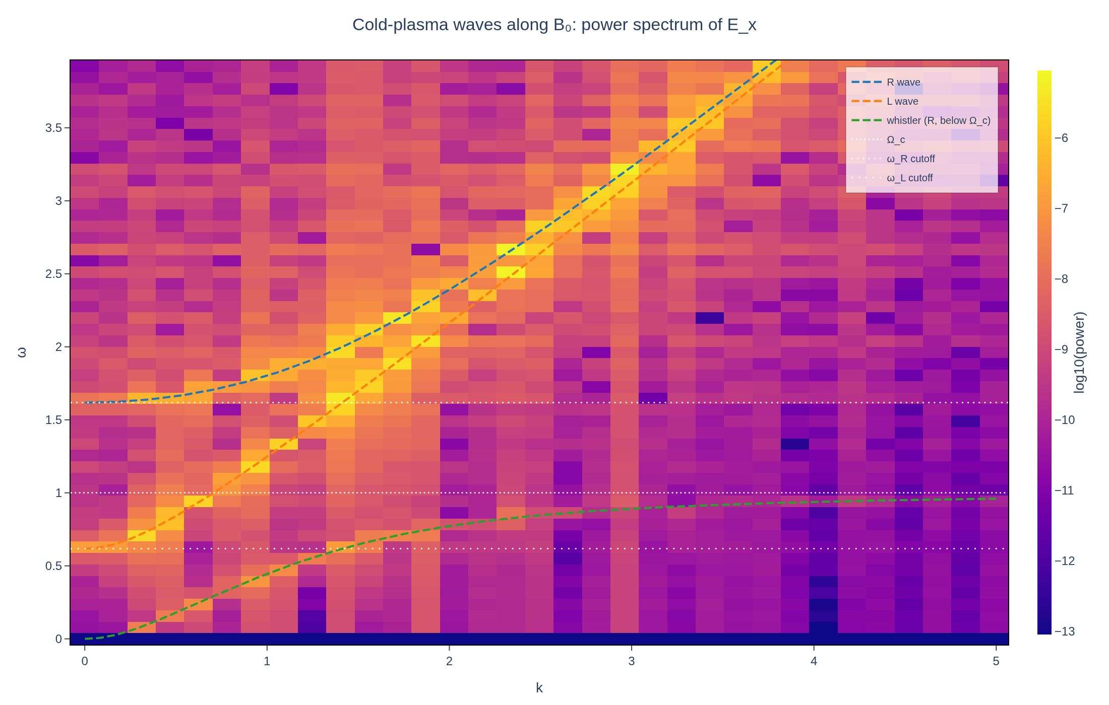
Broadband noise excites the right- and left-hand circularly polarized waves of a cold, magnetized electron plasma. The power spectrum of the transverse electric field shows the whistler branch below the cyclotron frequency and the two cutoffs, on top of the analytic cold-plasma dispersion relation.

Simulation geometry
Domain used in this run
The actual Cuboid geometry reconstructed from this run's metadata. Switch between the 3D view and physical-coordinate slices.
Domain
Cuboid
Mapping
Loading Cuboid…
Parameters
| Parameter | Value | Description |
|---|---|---|
| Loading parameters… | ||
Physical problem
Circularly polarized waves in a magnetized plasma
Broadband noise excites the right- and left-hand circularly polarized waves of a cold, magnetized electron plasma. The power spectrum of the transverse electric field shows the whistler branch below the cyclotron frequency and the two cutoffs, on top of the analytic cold-plasma dispersion relation.
PDEs solved by model:
Cold-plasma current:
Faraday's law:
Ampère's law:
where denotes an inhomogeneous background.
- Model
- ColdPlasma
- Domain
- Cuboid (r3=40)
- Grid
- 1 × 1 × 128
- FEEC degree
- 1 × 1 × 3
- Integrator
- Implicit
- Evolution
- 1,600 steps
- Visualization
- Plotly
Performance
Profiling
Struphy's built-in scope-profiler instruments every propagator, pusher and solver call — these are the real per-call timings from the run above.
Gantt (rank 0)
Region statistics
| Region | Count | Avg (s) | Min (s) | Max (s) | Total (s) |
|---|
Complete source
Simulation script
Requires Struphy with compiled kernels and Plotly. Run struphy compile once, then execute python cold-plasma-waves.py.
"""Electromagnetic waves along the magnetic field of a cold plasma, with Struphy's ColdPlasma model.

A cold electron fluid in a uniform magnetic field B0 = B0 e_z carries circularly polarized waves along
the field: the right-hand (R) wave with its whistler branch below the electron cyclotron frequency, and
the left-hand (L) wave. Both are cut off at low frequency, where the plasma reflects them. Broadband
noise in the transverse electric field excites all branches at once; the (k, omega) power spectrum of
E_x shows them, and is compared with the analytic cold-plasma dispersion relation.

Requires Struphy 3.3 with compiled kernels (`struphy compile`).
"""

import numpy as np
import plotly.graph_objects as go

from struphy import DerhamOptions, EnvironmentOptions, Simulation, Time, domains, equils, grids, perturbations
from struphy.diagnostics.diagn_tools import power_spectrum_2d
from struphy.models import ColdPlasma

# Plasma frequency equal to the cyclotron frequency (alpha = 1), and time in units of the inverse
# cyclotron frequency (epsilon = 1). The R cutoff is then at (1 + sqrt 5)/2 and the L cutoff at (sqrt 5 - 1)/2.
alpha, epsilon, n0, B0z = 1.0, 1.0, 1.0, 1.0
omega_R = 0.5 * (1.0 + np.sqrt(1.0 + 4.0 * alpha**2))
omega_L = 0.5 * (-1.0 + np.sqrt(1.0 + 4.0 * alpha**2))


def parallel_branches(k):
    """Positive frequencies of the cold electron plasma for k along B0, in units of the cyclotron frequency.

    With c = 1, k^2 = omega^2 - omega_p^2 omega / (omega -+ Omega_c) for the R (upper sign) and L waves,
    i.e. the cubic omega^3 -+ Omega_c omega^2 - (omega_p^2 + k^2) omega +- k^2 Omega_c = 0. The R cubic has
    two positive roots (the whistler below Omega_c and the R wave above omega_R), the L cubic one.
    (The longitudinal plasma oscillation, omega = omega_p, lives in E_z, which the noise leaves at zero.)
    """
    omega_c, omega_p2 = 1.0, alpha**2
    whistler, r_wave, l_wave = [], [], []
    for kk in k:
        r_roots = np.sort(np.roots([1.0, -omega_c, -(omega_p2 + kk**2), kk**2 * omega_c]).real)
        l_roots = np.sort(np.roots([1.0, omega_c, -(omega_p2 + kk**2), -(kk**2) * omega_c]).real)
        whistler.append(r_roots[-2])
        r_wave.append(r_roots[-1])
        l_wave.append(l_roots[-1])
    return {
        "R-wave": np.array(r_wave),
        "L-wave": np.array(l_wave),
        "whistler": np.array(whistler),
    }

model = ColdPlasma(alpha=alpha, epsilon=epsilon)
model.propagators.maxwell.options = model.propagators.maxwell.Options(algo="implicit")

# Broadband noise in both transverse components of E excites the R and L waves together.
for component in (0, 1):
    model.em_fields.e_field.add_perturbation(perturbations.Noise(amp=0.1, comp=component, seed=123))

domain = domains.Cuboid(r3=40.0)
grid = grids.TensorProductGrid(num_elements=(1, 1, 128))
derham_opts = DerhamOptions(degree=(1, 1, 3))
equil = equils.HomogenSlab(B0x=0.0, B0y=0.0, B0z=B0z, n0=n0)
time_opts = Time(dt=0.05, Tend=80.0)

env = EnvironmentOptions(out_folders="struphy_gallery_runs", sim_folder="cold_plasma_waves")
sim = Simulation(
    model=model,
    name="Cold-plasma waves along a magnetic field",
    description=(
        "Broadband noise excites the right- and left-hand circularly polarized waves of a cold, magnetized "
        "electron plasma. The power spectrum of the transverse electric field shows the whistler branch below "
        "the cyclotron frequency and the two cutoffs, on top of the analytic cold-plasma dispersion relation."
    ),
    env=env,
    time_opts=time_opts,
    domain=domain,
    equil=equil,
    grid=grid,
    derham_opts=derham_opts,
)


if __name__ == "__main__":
    from _gallery import export_profiling, merge_metadata, save_extra_figure, save_figure

    output = sim.run(profiling_activated=True)
    output.pproc(physical=True)

    omega, k, spectrum, _ = power_spectrum_2d(
        output.fields.em_fields.e_field,
        component=0,
        slice_at=[0, 0, None],
        physical=True,
        do_plot=False,
    )
    omega, k, spectrum = np.asarray(omega), np.asarray(k), np.asarray(spectrum)
    power = spectrum**2
    power /= power.max()

    # The analytic branches for propagation along B0.
    k_top, omega_top = 5.0, 4.0
    k_fine = np.linspace(1e-3, k_top, 400)
    branch_curves = parallel_branches(k_fine)

    # Read each branch off the spectrum: at every k, the frequency of the strongest power within a window
    # around the exact branch, and its relative distance from it.
    frequency_resolution = float(omega[1] - omega[0])
    errors = {}
    for name in branch_curves:
        deviations = []
        for column, kk in enumerate(k):
            if not 0.0 < kk <= k_top:
                continue
            target = float(np.interp(kk, k_fine, branch_curves[name]))
            window = np.flatnonzero(np.abs(omega - target) < 0.1 * target + 2.0 * frequency_resolution)
            if window.size and target <= omega_top:
                peak = omega[window[np.argmax(power[window, column])]]
                deviations.append(abs(peak / target - 1.0))
        errors[name] = float(np.median(deviations))
        print(f"{name}: median relative frequency error {errors[name]:.3f} over {len(deviations)} wavenumbers")
    if not all(np.isfinite(error) for error in errors.values()):
        raise RuntimeError("A wave branch could not be read off the spectrum")

    log_power = np.log10(np.clip(power, 1e-12, None))
    figure = go.Figure(
        go.Heatmap(
            x=k, y=omega, z=log_power, zmin=-8, zmax=0, colorscale="Plasma",
            colorbar={"title": {"text": "log₁₀ P"}},
            hovertemplate="k=%{x:.3f}<br>ω=%{y:.3f}<br>log₁₀ P=%{z:.2f}<extra></extra>",
        )
    )
    styles = {
        "R-wave": ("R wave", "#2a9d8f"),
        "L-wave": ("L wave", "#e9c46a"),
        "whistler": ("whistler (R, below Ω_c)", "#48cae4"),
    }
    for name, (label, color) in styles.items():
        figure.add_scatter(
            x=k_fine, y=branch_curves[name], mode="lines", name=label,
            line={"color": color, "width": 2.5, "dash": "dash"},
        )
    for level, label in ((1.0, "Ω_c"), (omega_R, "ω_R cutoff"), (omega_L, "ω_L cutoff")):
        figure.add_hline(y=level, line={"color": "rgba(255,255,255,0.55)", "width": 1, "dash": "dot"},
                         annotation_text=label, annotation_position="bottom right",
                         annotation_font_color="white")
    figure.update_layout(
        title="Cold-plasma waves along B₀: power spectrum of E_x",
        xaxis_title="k c / Ω_c", yaxis_title="ω / Ω_c", template="plotly_white", autosize=True,
        legend={"orientation": "h", "y": -0.18}, margin={"l": 75, "r": 40, "t": 80, "b": 110},
    )
    figure.update_xaxes(range=[0, k_top])
    figure.update_yaxes(range=[0, omega_top])
    save_figure(figure, "cold-plasma-waves", height=700)

    # Energy channels: the noise starts purely electric, then shares its energy with the magnetic field
    # and the electron current, while the sum stays constant.
    channels = {
        "electric_energy": ("electric", "#168aad"),
        "magnetic_energy": ("magnetic", "#d62828"),
        "kinetic_energy": ("electron current", "#f4a261"),
        "total_energy": ("total", "#264653"),
    }
    energies = {name: output.evaluate(name) for name in channels}
    time = energies["total_energy"].t.values
    total = energies["total_energy"].values
    relative_drift = float(np.max(np.abs(total / total[0] - 1.0)))
    print(f"Maximum relative drift of the total energy: {relative_drift:.2e}")
    energy_figure = go.Figure()
    for name, (label, color) in channels.items():
        energy_figure.add_scatter(x=time, y=energies[name].values, mode="lines", name=label,
                                  line={"color": color, "width": 3 if name == "total_energy" else 2})
    energy_figure.update_layout(
        title="Energy channels of the cold plasma", xaxis_title="t Ω_c", yaxis_title="energy [a.u.]",
        template="plotly_white", autosize=True, legend={"orientation": "h", "y": -0.2},
        margin={"l": 75, "r": 30, "t": 80, "b": 100},
    )
    figures = [
        save_extra_figure(
            energy_figure, "cold-plasma-waves", "energy",
            alt="Electric, magnetic and electron-current energy of the cold plasma against time, with their constant sum",
            caption=(
                "The initial noise is purely electric. Within a cyclotron period it is shared with the magnetic "
                "field and the kinetic energy of the electron current, while the total stays constant: its largest "
                f"relative change over the run is {relative_drift:.1e}. Each propagator of the splitting is a "
                "Crank–Nicolson step that conserves its share of the energy up to the tolerance of the linear solver."
            ),
        ),
    ]

    merge_metadata(
        "cold-plasma-waves",
        rWaveFrequencyError=errors["R-wave"],
        lWaveFrequencyError=errors["L-wave"],
        whistlerFrequencyError=errors["whistler"],
        relativeEnergyDrift=relative_drift,
        figures=figures,
        **export_profiling(sim, "cold-plasma-waves"),
    )
See the post-processing guide for more ways to inspect the result.