Overview

This is a fluid electromagnetic model for a cold plasma response. The

electron fluid is represented only through its current, so thermal pressure and kinetic velocity-space effects are omitted. It is useful as a reduced model between vacuum Maxwell and fully kinetic Vlasov-Maxwell dynamics.

Use cases

This model is appropriate for:

cold-plasma wave propagation studies
electromagnetic benchmarks with a fluid current response
regimes where thermal pressure can be neglected
algorithm verification for Maxwell plus current coupling

Governing equations

PDEs solved by model:

Cold-plasma current:

\frac{1}{n _{0}} \frac{\partial j}{\partial t} = \frac{1}{ε} E + \frac{1}{ε n _{0}} j \times B_{0}

Faraday's law:

\frac{\partial B}{\partial t} + \nabla \times E = 0

Ampère's law:

- \frac{\partial E}{\partial t} + \nabla \times B = \frac{α ^{2}}{ε} j

where $(n_{0}, B_{0})$ denotes an inhomogeneous background.

Normalization

Velocities are normalized with the speed of light and the fields satisfy

v^= c, E^= c B^.

The dimensionless plasma parameters are the cold-species $α = Ω^_{p} / Ω^_{c}$ and $ε = 1/ (Ω^_{c} t^)$ .

Discretization

Time integration is performed by the following propagators (in sequence):

Diagnostics

The following scalars are tracked during simulation:

Electric field energy: electric_energy
Magnetic field energy: magnetic_energy
Cold-current energy: kinetic_energy
Total energy: total_energy

Examples

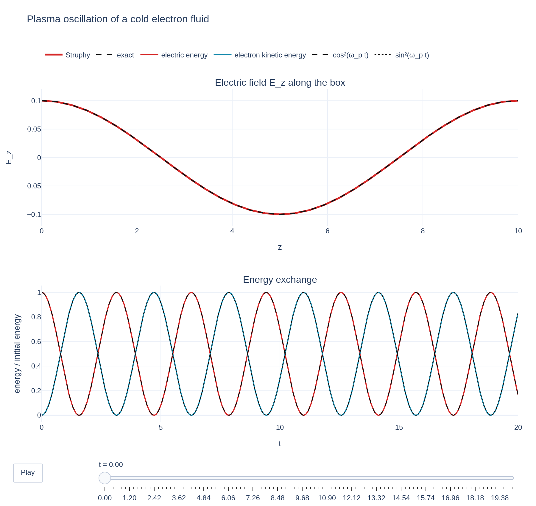
Cold-plasma oscillation

A cosine electric field along the magnetic field displaces a cold electron fluid, which oscillates at the plasma frequency. The field and flow energies trade places as cos² and sin² of the frequency, and the measured frequency follows the square root of the density. The initial electric field is $E_z(z,0)=0.1\cos(2\pi z/10),\qquad \mathbf{u}(z,0)=0,$ along $\mathbf{B}_0=\mathbf{e}_z$ . The density scan uses $n_0\in\{0.5,1,2,4\}$ with $\omega_p=\sqrt{n_0}$ .

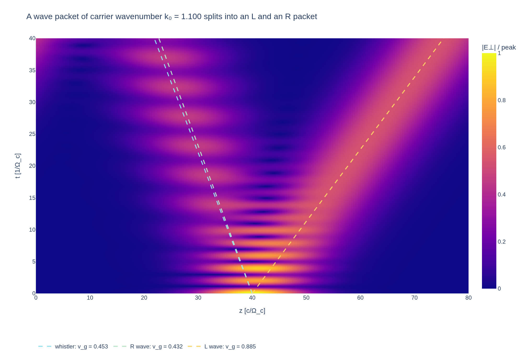
Cold-plasma wave packets

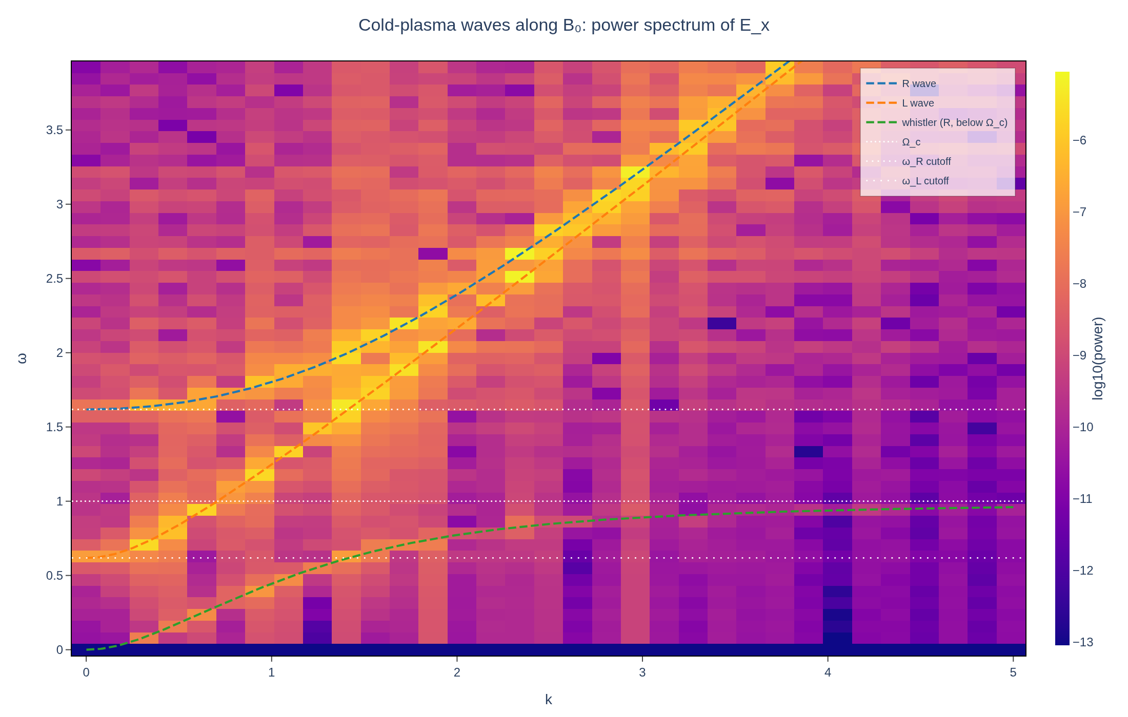
A Gaussian packet of circularly polarized electric field splits, in a magnetized cold plasma, into a fast L-wave packet and a slow, spreading R-wave packet that leave the launch point in opposite directions. Their speeds are the group velocities of the cold-plasma dispersion relation. The launch field is $\mathbf{E}(z,0)=0.05e^{-(z-40)^2/(2\cdot7^2)}(\cos(k_0z),-\sin(k_0z),0),$ with $k_0=2\pi\cdot14/80$ , $\mathbf{B}_0=\mathbf{e}_z$ and $n_0=1$ .

Cold-plasma waves along a magnetic field

Broadband noise excites the right- and left-hand circularly polarized waves of a cold, magnetized electron plasma. The power spectrum of the transverse electric field shows the whistler branch below the cyclotron frequency and the two cutoffs, on top of the analytic cold-plasma dispersion relation. The background parameters are $\mathbf{B}_0=\mathbf{e}_z,\qquad n_0=1,\qquad \alpha=\epsilon=1,$ with transverse electric coefficient-noise amplitude $0.1$ , $E_z(z,0)=0$ and periodic length $L_z=40$ .

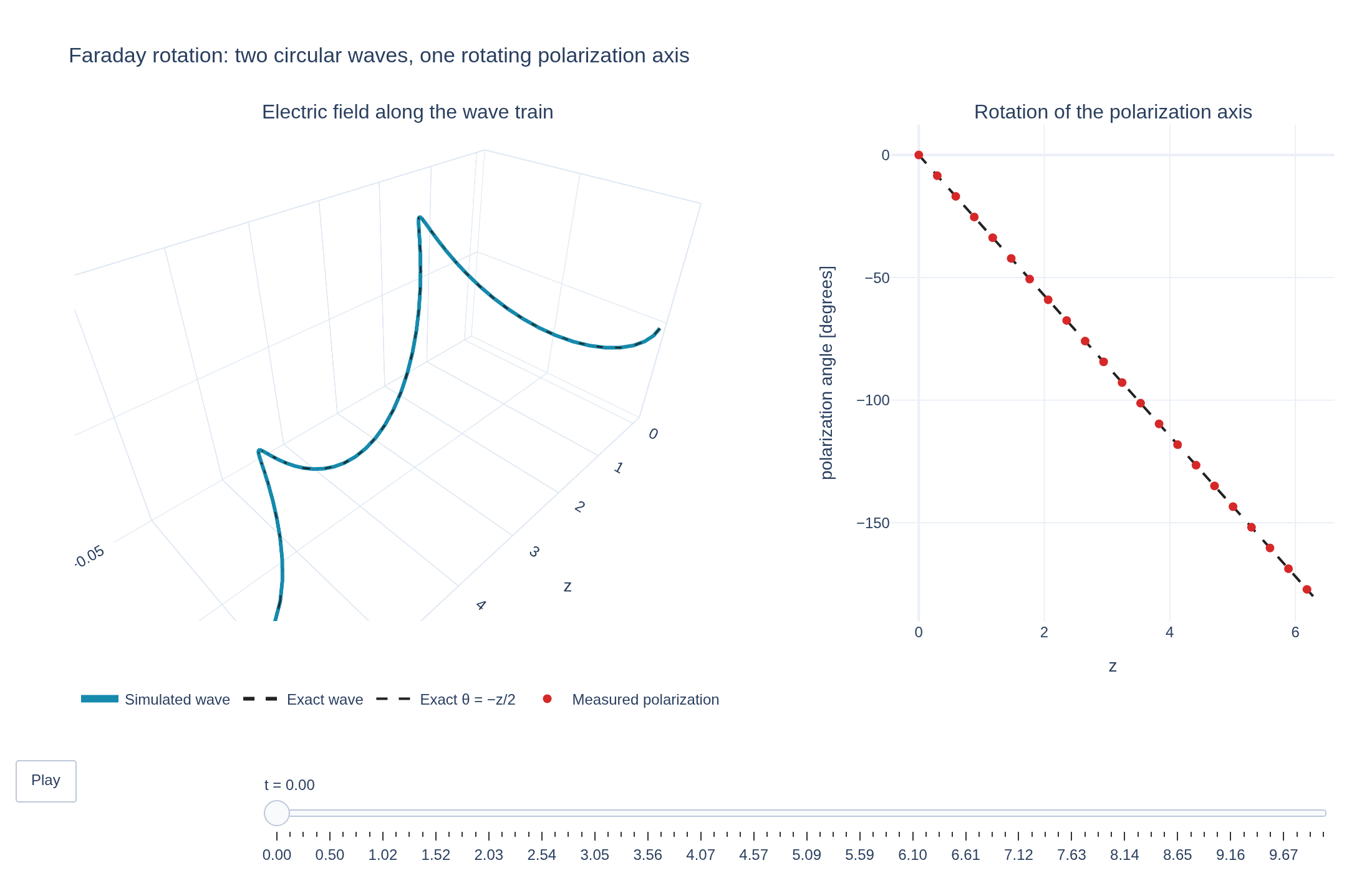
Faraday rotation in a magnetized plasma

Two circularly polarized waves of equal frequency and amplitude travel along the magnetic field. Their different wavelengths rotate the plane of their combined, linearly polarized electric field: the Faraday effect. This periodic example starts with the complete wave train, including its current and magnetic field. With $\omega=2.5$ , $B_0=1$ and $n_0=3.15$ , the wavenumbers are $k_1=1$ and $k_2=2$ . The electric field is $\mathbf{E}_\perp(z,t)=0.05\cos(1.5z-2.5t)(\cos(z/2),-\sin(z/2)),$ so the polarization axis rotates by $\theta(z)=-z/2$ , modulo $\pi$ , in this sign convention.

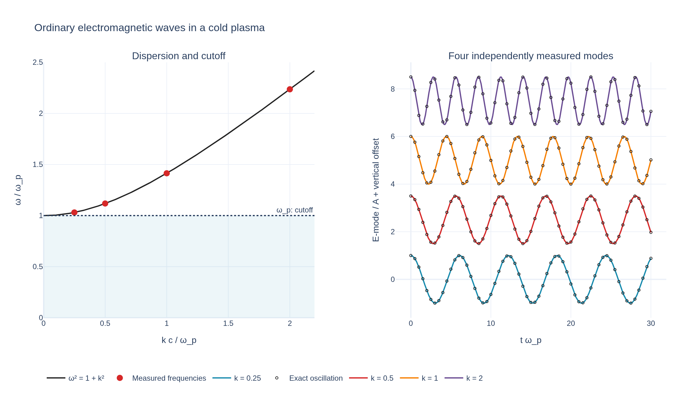
Ordinary waves and the plasma cutoff

Four ordinary electromagnetic waves oscillate across a uniform magnetic field. Their electric field is parallel to the background field, so the electrons feel no magnetic force in this polarization. Measured frequencies follow the cold-plasma dispersion relation $\omega^2=\omega_p^2+c^2k^2,\qquad \omega_p=c=1.$ Initially $E_z(x,0)=0.02\sum_{n\in\{1,2,4,8\}}\cos(nx/4)$ and the magnetic perturbation and current vanish. The dispersion curve approaches the plasma-frequency cutoff as the wavelength grows; below it, a uniform cold plasma has no propagating ordinary mode.