ViscoResistiveMHD · Resistive MHD
Resistive diffusion of a magnetic field
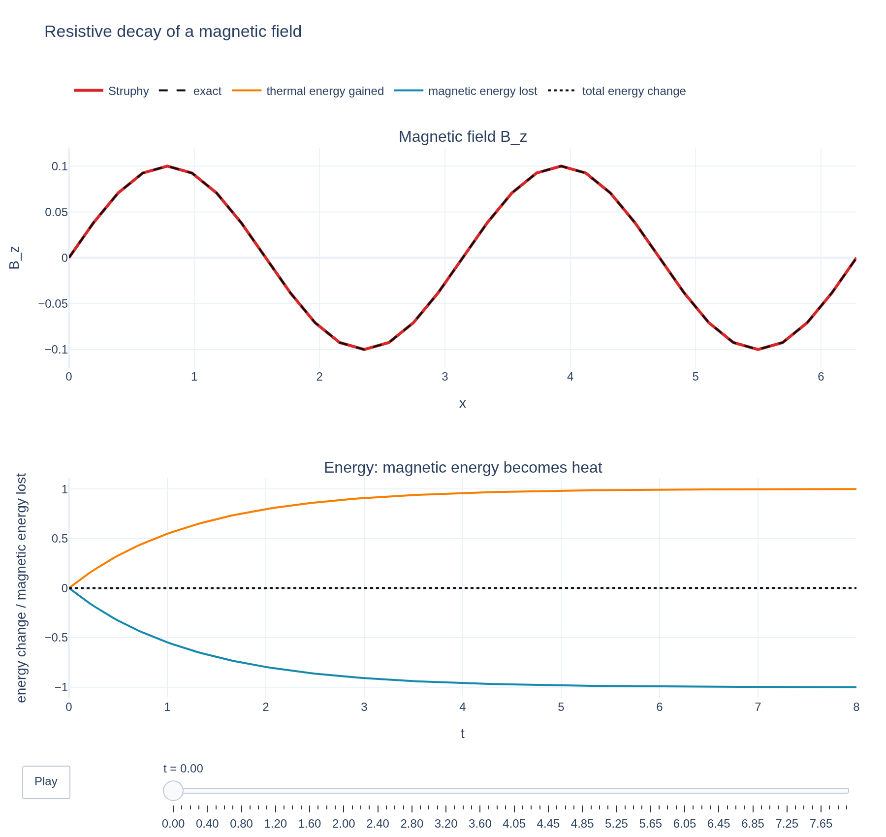
A sinusoidal magnetic field in a resistive plasma at rest decays without changing shape, at the rate η k². Struphy's variational discretization converts the lost magnetic energy into thermal energy and keeps the total energy constant.
Loading interactive figure…
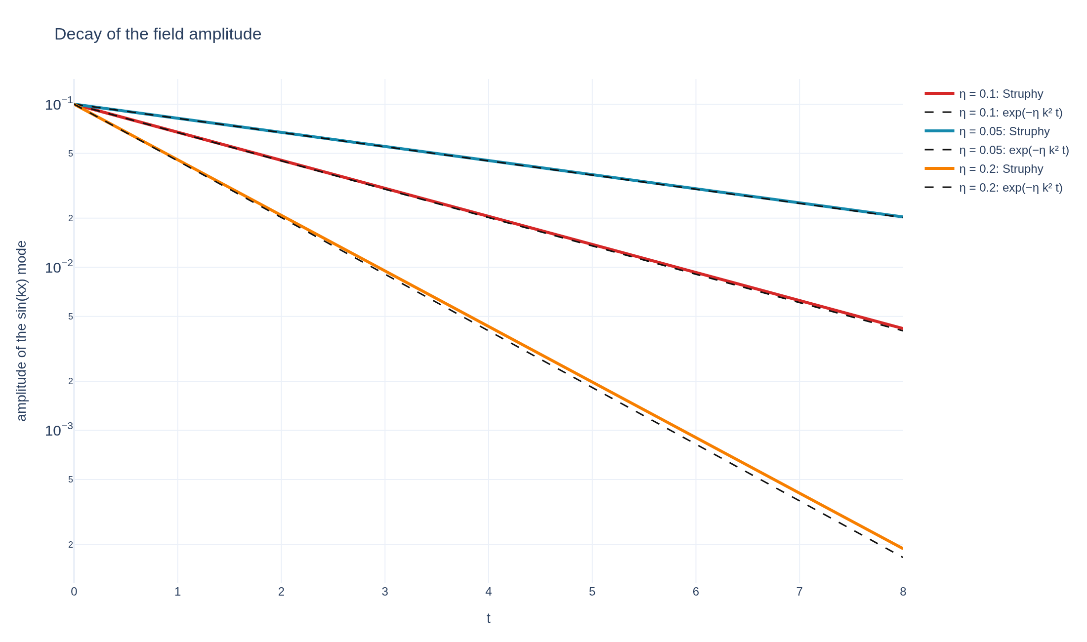
Loading interactive figure…
Physical problem
A field that leaks away
PDEs solved by model:
Continuity:
Momentum:
Entropy:
Induction:
where the internal energy per unit mass is , and and are artificial viscosity and resistivity coefficients.
Simulation geometry
Domain used in this run
The actual Cuboid geometry reconstructed from this run's metadata. Switch between the 3D view and physical-coordinate slices.
Domain
Cuboid
Mapping
Loading Cuboid…
Parameters
| Parameter | Value | Description |
|---|---|---|
| Loading parameters… | ||
Performance
Profiling
Struphy's built-in scope-profiler instruments every propagator, pusher and solver call — these are the real per-call timings from the run above.
Durations
Gantt (rank 0)
Region statistics
| Region | Count | Avg (s) | Min (s) | Max (s) | Total (s) |
|---|
Complete source
Simulation script
Requires Struphy with compiled kernels and Plotly. Run struphy compile once, then execute python resistive-diffusion.py.
"""Resistive diffusion of a magnetic field, with Struphy's ViscoResistiveMHD model.

In a resistive plasma at rest the magnetic field obeys a diffusion equation, dB/dt = eta B'', where eta is the resistivity.
A sinusoidal field B_z = B_0 sin(k x) therefore decays without changing its shape, as exp(-eta k^2 t), and the magnetic energy
decays twice as fast, as exp(-2 eta k^2 t). Struphy's variational discretization turns the lost magnetic energy into
thermal energy (Ohmic heating) and keeps the total energy constant to the accuracy of its nonlinear solver. The field is weak, so that
the pressure gradient it produces sets only a negligible flow. A scan over three resistivities confirms the rate.

Requires Struphy 3.3 with compiled kernels (`struphy compile`).
"""

import numpy as np
import plotly.graph_objects as go

from struphy import (
    DerhamOptions,
    EnvironmentOptions,
    FieldsBackground,
    Simulation,
    Time,
    domains,
    equils,
    grids,
    perturbations,
)
from struphy.linear_algebra.solver import NonlinearSolverParameters
from struphy.models import ViscoResistiveMHD

length = 2 * np.pi
mode_number = 2
wavenumber = 2 * np.pi * mode_number / length
amplitude = 0.1
resistivities = (0.05, 0.1, 0.2)  # the scan; the example itself is the eta = 0.1 run
time_opts = Time(dt=0.05, Tend=8.0, split_algo="LieTrotter")
grid = grids.TensorProductGrid(num_elements=(32, 1, 1))
derham_opts = DerhamOptions(degree=(3, 1, 1))
domain = domains.Cuboid(l1=0.0, r1=length, l2=0.0, r2=1.0, l3=0.0, r3=1.0)
equil = equils.HomogenSlab(B0z=1.0, n0=1.0, beta=2.0)


class CompatibleNonlinearSolverParameters(NonlinearSolverParameters):
    """Bridge Struphy code paths that use both attribute and mapping access."""

    def __getitem__(self, key):
        return getattr(self, key)


def make_simulation(eta, folder, **extra):
    """The resistive-MHD model with resistivity eta and a sine mode in the out-of-plane field B_z."""
    model = ViscoResistiveMHD(with_viscosity=False, with_resistivity=True)
    model.propagators.variat_dens.options = model.propagators.variat_dens.Options(model="full")
    model.propagators.variat_resist.options = model.propagators.variat_resist.Options(
        model="full",
        eta=eta,
        nonlin_solver=CompatibleNonlinearSolverParameters(type="Newton"),
    )
    # Logical 3-forms include det(DF) = length, giving a physical density 1 and a uniform thermal pressure.
    volume = length
    model.mhd.density.add_background(FieldsBackground(values=(volume,)))
    model.mhd.entropy.add_background(FieldsBackground(values=(0.6 * volume,)))
    model.mhd.velocity.add_background(FieldsBackground(values=(0.0, 0.0, 0.0)))
    model.em_fields.b_field.add_background(FieldsBackground(values=(0.0, 0.0, 0.0)))
    model.em_fields.b_field.add_perturbation(
        perturbations.ModesSin(ls=(mode_number,), amps=(amplitude,), Lx=length, comp=2, given_in_basis="physical")
    )
    return Simulation(
        model=model,
        env=EnvironmentOptions(out_folders="struphy_gallery_runs", sim_folder=folder),
        time_opts=time_opts,
        domain=domain,
        equil=equil,
        grid=grid,
        derham_opts=derham_opts,
        **extra,
    )


sim = make_simulation(
    0.1,
    "resistive_diffusion",
    name="Resistive diffusion of a magnetic field",
    description=(
        "A sinusoidal magnetic field in a resistive plasma at rest decays without changing shape, at the rate "
        "η k². Struphy's variational discretization converts the lost magnetic energy into thermal energy and keeps "
        "the total energy constant."
    ),
)


def field_profile(run):
    """Time, position and B_z(t, x) of a post-processed run."""
    b_z = run.evaluate("em_fields/b_field_xyz").isel(component=2, e2=0, e3=0)
    return b_z.t.values, b_z.e1.values * length, b_z.values


def mode_amplitude(x, values):
    """Amplitude of the sin(k x) mode, from the periodic grid points (the last repeats the first)."""
    return 2.0 * np.mean(values[:, :-1] * np.sin(wavenumber * x[:-1]), axis=1)


if __name__ == "__main__":
    from plotly.subplots import make_subplots

    from _gallery import export_profiling, is_root, merge_metadata, save_extra_figure, save_figure

    runs = {0.1: sim.run(profiling_activated=True)}
    for eta in resistivities:
        if eta != 0.1:
            runs[eta] = make_simulation(eta, f"resistive_diffusion_eta{eta}").run()
    for run in runs.values():
        run.pproc(physical=True)

    amplitudes, fitted = {}, {}
    for eta, run in runs.items():
        times, x, values = field_profile(run)
        amplitudes[eta] = mode_amplitude(x, values)
        fitted[eta] = float(-np.polyfit(times, np.log(np.abs(amplitudes[eta])), 1)[0])
    exact_rate = {eta: eta * wavenumber**2 for eta in runs}
    if not all(np.isfinite(list(fitted.values()))):
        raise RuntimeError("A decay rate could not be fitted")
    if is_root():
        for eta in runs:
            print(f"eta = {eta}: decay rate {fitted[eta]:.4f} (exact {exact_rate[eta]:.4f})")

    run = runs[0.1]
    eta_main = 0.1
    times, x, values = field_profile(run)
    magnetic = np.asarray(run.scalars["en_mag"])
    thermal = np.asarray(run.scalars["en_thermo"])
    total = np.asarray(run.scalars["en_tot"])
    scalar_times = np.asarray(run.time)[: len(total)]
    energy_drift = float(np.max(np.abs(total / total[0] - 1.0)))
    print(f"Maximum relative drift of the total energy: {energy_drift:.2e}")

    def profile_traces(index):
        decay = np.exp(-exact_rate[eta_main] * times[index])
        return [
            go.Scatter(x=x, y=values[index], mode="lines", name="Struphy", line={"color": "#d62828", "width": 3}),
            go.Scatter(x=x, y=amplitude * decay * np.sin(wavenumber * x), mode="lines", name="exact",
                       line={"color": "#111", "width": 2, "dash": "dash"}),
        ]

    picks = np.unique(np.linspace(0, len(times) - 1, min(80, len(times)), dtype=int))
    figure = make_subplots(rows=2, cols=1, vertical_spacing=0.2,
                           subplot_titles=("Magnetic field B_z", "Energy: magnetic energy becomes heat"))
    for trace in profile_traces(0):
        figure.add_trace(trace, row=1, col=1)
    figure.add_scatter(x=scalar_times, y=(thermal - thermal[0]) / (magnetic[0] - magnetic[-1]), mode="lines",
                       name="thermal energy gained", line={"color": "#f77f00", "width": 2}, row=2, col=1)
    figure.add_scatter(x=scalar_times, y=(magnetic - magnetic[0]) / (magnetic[0] - magnetic[-1]), mode="lines",
                       name="magnetic energy lost", line={"color": "#168aad", "width": 2}, row=2, col=1)
    figure.add_scatter(x=scalar_times, y=(total - total[0]) / (magnetic[0] - magnetic[-1]), mode="lines",
                       name="total energy change", line={"color": "#111", "width": 2, "dash": "dot"}, row=2, col=1)
    figure.frames = [go.Frame(name=f"{times[i]:.2f}", data=profile_traces(i), traces=[0, 1]) for i in picks]
    figure.update_layout(
        title="Resistive decay of a magnetic field", template="plotly_white",
        margin={"l": 70, "r": 30, "t": 150, "b": 140}, title_y=0.97, legend={"orientation": "h", "y": 1.13},
        updatemenus=[{"type": "buttons", "showactive": False, "x": 0, "y": -0.12,
                      "buttons": [{"label": "Play", "method": "animate", "args": [None, {"frame": {"duration": 60, "redraw": False}, "transition": {"duration": 0}, "fromcurrent": True}]}]}],
        sliders=[{"active": 0, "x": 0.12, "len": 0.88, "y": -0.07, "currentvalue": {"prefix": "t = "},
                  "steps": [{"args": [[frame.name], {"frame": {"duration": 0, "redraw": False}, "transition": {"duration": 0}, "mode": "immediate"}], "label": frame.name, "method": "animate"} for frame in figure.frames]}],
    )
    figure.update_xaxes(title_text="x", range=[0, length], row=1, col=1)
    figure.update_yaxes(title_text="B_z", range=[-1.2 * amplitude, 1.2 * amplitude], row=1, col=1)
    figure.update_xaxes(title_text="t", row=2, col=1)
    figure.update_yaxes(title_text="energy change / magnetic energy lost", row=2, col=1)
    save_figure(figure, "resistive-diffusion", width=900, height=850)

    colors = {0.05: "#168aad", 0.1: "#d62828", 0.2: "#f77f00"}
    decay = go.Figure()
    for eta, amp in amplitudes.items():
        decay.add_scatter(x=times, y=np.abs(amp), mode="lines", name=f"η = {eta}: Struphy",
                          line={"color": colors[eta], "width": 3})
        decay.add_scatter(x=times, y=amplitude * np.exp(-exact_rate[eta] * times), mode="lines",
                          name=f"η = {eta}: exp(−η k² t)", line={"color": "#111", "width": 1.5, "dash": "dash"})
    decay.update_layout(
        title="Decay of the field amplitude", template="plotly_white", autosize=True,
        xaxis_title="t", yaxis_title="amplitude of the sin(kx) mode", yaxis_type="log",
        margin={"l": 75, "r": 30, "t": 80, "b": 60},
    )
    figures = [
        save_extra_figure(
            decay, "resistive-diffusion", "decay",
            alt="Decay of the amplitude of a magnetic field mode at three resistivities, on the exact exponentials",
            caption=(
                "The amplitude of the field mode at three resistivities, on log axes where the exact decay exp(−η k² t) "
                "is a straight line. The fitted rates differ from η k² by "
                + ", ".join(f"{100 * (fitted[eta] / exact_rate[eta] - 1):+.1f} % (η = {eta})" for eta in runs)
                + "."
            ),
        ),
    ]

    merge_metadata(
        "resistive-diffusion",
        wavenumber=wavenumber,
        decayRates={str(eta): {"measured": fitted[eta], "exact": exact_rate[eta]} for eta in runs},
        maxEnergyDrift=energy_drift,
        figures=figures,
        **export_profiling(sim, "resistive-diffusion"),
    )
See the post-processing guide for more ways to inspect the result.