ViscoResistiveMHD · Magnetic reconnection
Resistive magnetic X-point
A periodic magnetic X-point is squeezed by an incompressible strain and evolved with Struphy's nonlinear visco-resistive MHD model. Finite resistivity supports an out-of-plane electric field at the null, changes the flux connecting the X- and O-points, and converts magnetic energy into internal energy while the compatible FEEC discretization controls div B.
Loading interactive figure…
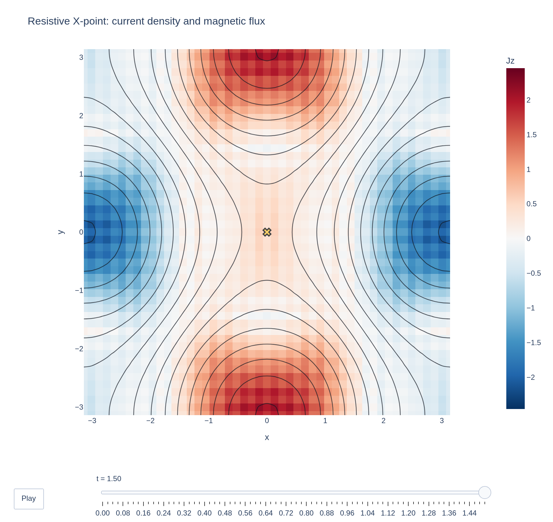
Loading interactive figure…
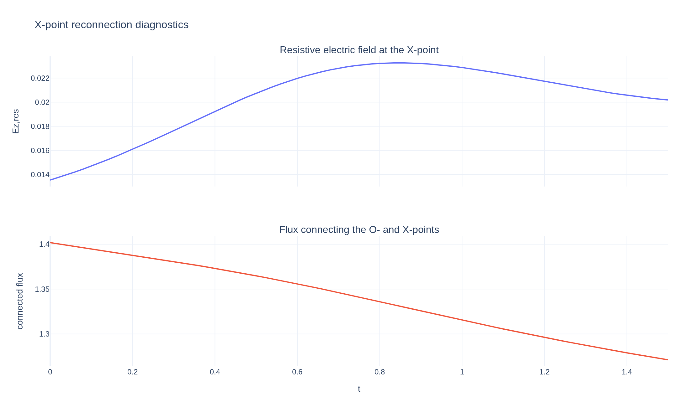
Loading interactive figure…
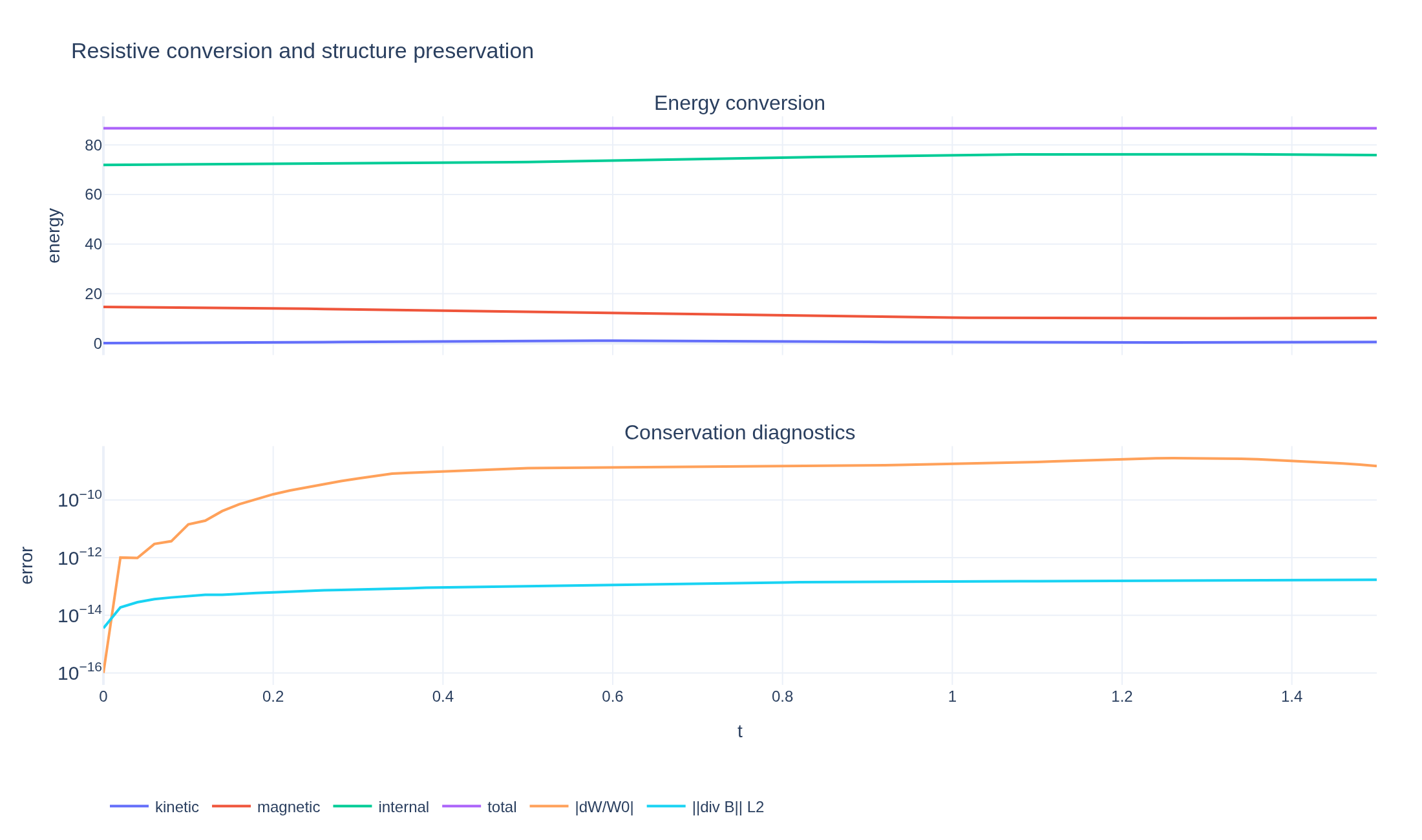
Physical problem
Resistive relaxation of a driven magnetic null
A periodic magnetic X-point is squeezed by an incompressible strain and evolved with Struphy's nonlinear visco-resistive MHD model. Finite resistivity supports an out-of-plane electric field at the null, changes the flux connecting the X- and O-points, and converts magnetic energy into internal energy while the compatible FEEC discretization controls div B.
PDEs solved by model:
Continuity:
Momentum:
Entropy:
Induction:
where the internal energy per unit mass is , and and are artificial viscosity and resistivity coefficients.
Simulation geometry
Domain used in this run
The actual Cuboid geometry reconstructed from this run's metadata. Switch between the 3D view and physical-coordinate slices.
Domain
Cuboid
Mapping
Loading Cuboid…
Parameters
| Parameter | Value | Description |
|---|---|---|
| Loading parameters… | ||
- Model
- ViscoResistiveMHD
- Grid
- 24 × 24 × 1
- FEEC degree
- 2 × 2 × 1
- Evolution
- 75 steps
- Visualization
- Plotly
Performance
Profiling
Struphy's built-in scope-profiler instruments every propagator, pusher and solver call — these are the real per-call timings from the run above.
Durations
Gantt (rank 0)
Region statistics
| Region | Count | Avg (s) | Min (s) | Max (s) | Total (s) |
|---|
Complete source
Simulation script
Requires Struphy with compiled kernels and Plotly. Run struphy compile once, then execute python resistive-x-point.py.
"""Resistive relaxation of a driven magnetic X-point in two-dimensional MHD.

The periodic flux A_z = cos(x) - lambda cos(y) gives
B = (d_y A_z, -d_x A_z, 0). For positive lambda the null at the origin is an
X-point. A small incompressible strain drives flux towards it and finite
resistivity permits reconnection.

Requires Struphy 3.3 with compiled kernels (``struphy compile``).
"""

import numpy as np
import plotly.graph_objects as go

from struphy import (
    DerhamOptions,
    EnvironmentOptions,
    FieldsBackground,
    Simulation,
    Time,
    domains,
    equils,
    grids,
    perturbations,
)
from struphy.linear_algebra.solver import NonlinearSolverParameters
from struphy.models import ViscoResistiveMHD

period = 2 * np.pi
box_min, box_max = -np.pi, np.pi
flux_asymmetry = 0.7
resistivity = 0.05
drive_amplitude = 0.08


class CompatibleNonlinearSolverParameters(NonlinearSolverParameters):
    """Bridge Struphy code paths that use both attribute and mapping access."""

    def __getitem__(self, key):
        return getattr(self, key)


model = ViscoResistiveMHD(with_viscosity=False, with_resistivity=True)
model.propagators.variat_dens.options = model.propagators.variat_dens.Options(model="full")
model.propagators.variat_resist.options = model.propagators.variat_resist.Options(
    model="full",
    eta=resistivity,
    nonlin_solver=CompatibleNonlinearSolverParameters(type="Newton"),
)

domain = domains.Cuboid(l1=box_min, r1=box_max, l2=box_min, r2=box_max, l3=0.0, r3=1.0)
grid = grids.TensorProductGrid(num_elements=(24, 24, 1))
derham_opts = DerhamOptions(degree=(2, 2, 1))
time_opts = Time(dt=0.02, Tend=1.5, split_algo="LieTrotter")
equil = equils.HomogenSlab(B0z=1.0, n0=1.0, beta=2.0)

# Logical 3-forms include det(DF) = (2*pi)^2, giving physical rho = 1 and
# uniform entropy density. The evolved magnetic field itself has no guide field.
volume = period**2
model.mhd.density.add_background(FieldsBackground(values=(volume,)))
model.mhd.entropy.add_background(FieldsBackground(values=(0.6 * volume,)))
model.mhd.velocity.add_background(FieldsBackground(values=(0.0, 0.0, 0.0)))
model.em_fields.b_field.add_background(FieldsBackground(values=(0.0, 0.0, 0.0)))
model.em_fields.b_field.add_perturbation(
    perturbations.ModesSin(
        ms=(1,), amps=(flux_asymmetry,), Ly=period, comp=0, given_in_basis="physical",
    )
)
model.em_fields.b_field.add_perturbation(
    perturbations.ModesSin(
        ls=(1,), amps=(1.0,), Lx=period, comp=1, given_in_basis="physical",
    )
)

# Divergence-free strain u = (-u0 sin(x) cos(y), u0 cos(x) sin(y), 0).
model.mhd.velocity.add_perturbation(
    perturbations.ModesSinCos(
        ls=(1,), ms=(1,), amps=(-drive_amplitude,), Lx=period, Ly=period,
        comp=0, given_in_basis="physical",
    )
)
model.mhd.velocity.add_perturbation(
    perturbations.ModesCosSin(
        ls=(1,), ms=(1,), amps=(drive_amplitude,), Lx=period, Ly=period,
        comp=1, given_in_basis="physical",
    )
)

env = EnvironmentOptions(out_folders="struphy_gallery_runs", sim_folder="resistive_x_point", max_runtime=3600)
sim = Simulation(
    model=model,
    name="Resistive magnetic X-point",
    description=(
        "A periodic magnetic X-point is squeezed by an incompressible strain and evolved "
        "with Struphy's nonlinear visco-resistive MHD model. Finite resistivity supports an out-of-plane "
        "electric field at the null, changes the flux connecting the X- and O-points, and converts magnetic "
        "energy into internal energy while the compatible FEEC discretization controls div B."
    ),
    env=env,
    time_opts=time_opts,
    domain=domain,
    equil=equil,
    grid=grid,
    derham_opts=derham_opts,
)


if __name__ == "__main__":
    from plotly.subplots import make_subplots

    from _gallery import export_profiling, merge_metadata, save_extra_figure, save_figure

    output = sim.run(profiling_activated=True)
    output.pproc(physical=True, celldivide=2)
    if not all(bool(np.isfinite(value).all()) for value in output.scalars.values()):
        raise RuntimeError("Non-finite X-point diagnostics: refusing to publish the run")

    b = output.evaluate("em_fields/b_field_xyz").isel(e3=0)
    rho = output.evaluate("mhd/density_xyz").isel(e3=0).squeeze(drop=True)
    times = np.asarray(b.t.values)
    if times[-1] < time_opts.Tend - 0.5 * time_opts.dt or float(rho.min()) <= 0:
        raise RuntimeError("Incomplete X-point evolution or non-positive density")

    x = np.asarray(b.X)[:, 0]
    y = np.asarray(b.Y)[0, :]
    bx, by = (b.isel(component=index).transpose("t", "e1", "e2").values for index in (0, 1))
    nx, ny = (
        count - 1 if abs(coordinates[-1] - coordinates[0] - period) < 1e-6 * period else count
        for count, coordinates in ((len(x), x), (len(y), y))
    )
    kx = 2 * np.pi * np.fft.fftfreq(nx, d=period / nx)[:, None]
    ky = 2 * np.pi * np.fft.fftfreq(ny, d=period / ny)[None, :]
    k2 = np.where((kx == 0) & (ky == 0), 1.0, kx**2 + ky**2)
    bx_hat, by_hat = (np.fft.fft2(field[:, :nx, :ny], axes=(1, 2)) for field in (bx, by))
    curl_hat = 1j * (kx * by_hat - ky * bx_hat)
    flux = np.fft.ifft2(curl_hat / k2, axes=(1, 2)).real
    current = np.fft.ifft2(curl_hat, axes=(1, 2)).real
    flux = np.pad(flux, ((0, 0), (0, len(x) - nx), (0, len(y) - ny)), mode="wrap")
    current = np.pad(current, ((0, 0), (0, len(x) - nx), (0, len(y) - ny)), mode="wrap")
    if not (np.isfinite(flux).all() and np.isfinite(current).all()):
        raise RuntimeError("Non-finite X-point field reconstruction")

    ix, iy = int(np.argmin(np.abs(x))), int(np.argmin(np.abs(y)))
    iy_o = int(np.argmin(np.abs(y - box_min)))
    current_at_x = current[:, ix, iy]
    reconnection_rate = resistivity * current_at_x
    connected_flux = flux[:, ix, iy_o] - flux[:, ix, iy]
    current_limit = float(np.percentile(np.abs(current), 99.5))
    flux_limit = float(np.max(np.abs(flux)))
    flux_levels = {"start": -flux_limit, "end": flux_limit, "size": 2 * flux_limit / 18}

    def field_traces(index):
        return [
            go.Heatmap(
                x=x, y=y, z=current[index].T, zmin=-current_limit, zmax=current_limit,
                colorscale="RdBu_r", colorbar={"title": "Jz"},
                hovertemplate="x=%{x:.3f}<br>y=%{y:.3f}<br>Jz=%{z:.4f}<extra></extra>",
            ),
            go.Contour(
                x=x, y=y, z=flux[index].T, contours={"coloring": "none", **flux_levels},
                line={"color": "rgba(20,25,35,.72)", "width": 1.2},
                showscale=False, showlegend=False, hoverinfo="skip",
            ),
            go.Scatter(
                x=[0.0], y=[0.0], mode="markers", name="X-point",
                marker={"symbol": "x", "size": 11, "color": "#ffd166", "line": {"width": 2}},
                showlegend=False, hovertemplate="magnetic null<extra></extra>",
            ),
        ]

    picks = np.unique(np.linspace(0, len(times) - 1, min(81, len(times)), dtype=int))
    figure = go.Figure(
        data=field_traces(0),
        frames=[go.Frame(name=f"{times[i]:.2f}", data=field_traces(i), traces=[0, 1, 2]) for i in picks],
    )
    figure.update_layout(
        title="Resistive X-point: current density and magnetic flux", template="plotly_white",
        margin={"l": 70, "r": 70, "t": 80, "b": 130}, showlegend=False,
        updatemenus=[{
            "type": "buttons", "showactive": False, "x": 0, "y": -0.2,
            "buttons": [{"label": "Play", "method": "animate", "args": [None, {
                "frame": {"duration": 55, "redraw": True}, "transition": {"duration": 0}, "fromcurrent": True,
            }]}],
        }],
        sliders=[{
            "active": 0, "x": 0.12, "len": 0.88, "y": -0.12, "currentvalue": {"prefix": "t = "},
            "steps": [{
                "args": [[frame.name], {
                    "frame": {"duration": 0, "redraw": True}, "transition": {"duration": 0}, "mode": "immediate",
                }],
                "label": frame.name, "method": "animate",
            } for frame in figure.frames],
        }],
    )
    figure.update_xaxes(title_text="x", range=[box_min, box_max], constrain="domain")
    figure.update_yaxes(title_text="y", range=[box_min, box_max], scaleanchor="x", scaleratio=1)
    save_figure(
        figure, "resistive-x-point", width=900, height=850,
        static_data=field_traces(len(times) - 1), static_active=len(figure.frames) - 1,
    )

    reconnection = make_subplots(
        rows=2, cols=1, shared_xaxes=True, vertical_spacing=0.16,
        subplot_titles=("Resistive electric field at the X-point", "Flux connecting the O- and X-points"),
    )
    reconnection.add_scatter(x=times, y=reconnection_rate, mode="lines", name="eta Jz(X)", row=1, col=1)
    reconnection.add_scatter(x=times, y=connected_flux, mode="lines", name="Az(O) - Az(X)", row=2, col=1)
    reconnection.update_yaxes(title_text="Ez,res", row=1, col=1)
    reconnection.update_yaxes(title_text="connected flux", row=2, col=1)
    reconnection.update_xaxes(title_text="t", row=2, col=1)
    reconnection.update_layout(
        title="X-point reconnection diagnostics", template="plotly_white", showlegend=False,
        margin={"l": 80, "r": 35, "t": 90, "b": 65},
    )

    scalars = output.scalars
    total_energy = scalars.en_tot
    energy_drift = np.abs(total_energy / total_energy.isel(t=0) - 1.0)
    divergence = np.sqrt(np.maximum(scalars.tot_div_B, 0.0))
    conservation = make_subplots(
        rows=2, cols=1, shared_xaxes=True, vertical_spacing=0.16,
        subplot_titles=("Energy conversion", "Conservation diagnostics"),
    )
    for key, label in (
        ("en_U", "kinetic"), ("en_mag", "magnetic"),
        ("en_thermo", "internal"), ("en_tot", "total"),
    ):
        conservation.add_scatter(x=scalars.t.values, y=scalars[key].values, mode="lines", name=label, row=1, col=1)
    conservation.add_scatter(
        x=scalars.t.values, y=np.maximum(energy_drift.values, 1e-16),
        mode="lines", name="|dW/W0|", row=2, col=1,
    )
    conservation.add_scatter(
        x=scalars.t.values, y=np.maximum(divergence.values, 1e-16),
        mode="lines", name="||div B|| L2", row=2, col=1,
    )
    conservation.update_yaxes(title_text="energy", row=1, col=1)
    conservation.update_yaxes(title_text="error", type="log", row=2, col=1)
    conservation.update_xaxes(title_text="t", row=2, col=1)
    conservation.update_layout(
        title="Resistive conversion and structure preservation", template="plotly_white",
        margin={"l": 80, "r": 35, "t": 90, "b": 75}, legend={"orientation": "h", "y": -0.18},
    )

    figures = [
        save_extra_figure(
            reconnection, "resistive-x-point", "reconnection",
            alt="Resistive electric field and connected magnetic flux at the X-point",
            caption=(
                "The resistive contribution eta Jz at the central null is the reconnection electric field in "
                "this symmetric two-dimensional setup. The lower panel tracks the flux difference between "
                "the neighbouring O-point and the X-point."
            ),
        ),
        save_extra_figure(
            conservation, "resistive-x-point", "conservation",
            alt="MHD energy conversion, total-energy error and magnetic-divergence norm",
            caption=(
                "Resistivity converts magnetic energy into internal energy. Total-energy change and the "
                "discrete L2 norm of div B monitor the numerical evolution."
            ),
        ),
    ]
    merge_metadata(
        "resistive-x-point",
        finalTime=float(times[-1]), resistivity=resistivity,
        peakReconnectionRate=float(np.max(np.abs(reconnection_rate))),
        connectedFluxChange=float(connected_flux[-1] - connected_flux[0]),
        maxEnergyDrift=float(energy_drift.max()), maxDivB=float(divergence.max()),
        minDensity=float(rho.min()), figures=figures,
        **export_profiling(sim, "resistive-x-point"),
    )
See the post-processing guide for more ways to inspect the result.