Vlasov · Particle drifts
Grad-B drift of charged particles
Charged particles gyrate more tightly on the stronger-field side of an orbit, producing a drift perpendicular to both the magnetic field and its gradient. Three test ions demonstrate how the drift grows with perpendicular kinetic energy. The magnetic field is externally prescribed; its straight field lines exclude curvature drift. Here and the ions start at with , and . Their measured drift is compared with the guiding-center approximation .
Loading interactive figure…
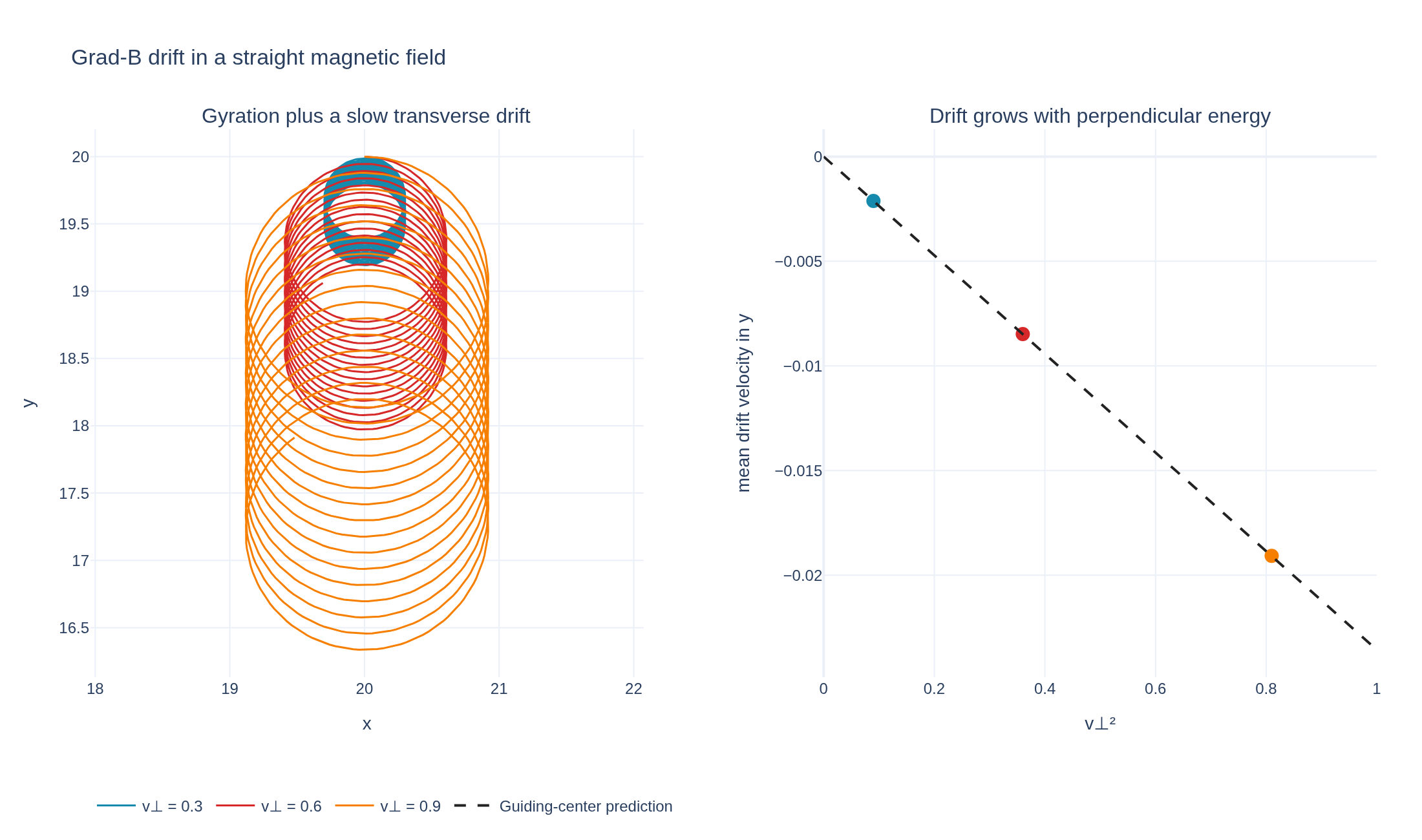
Loading interactive figure…
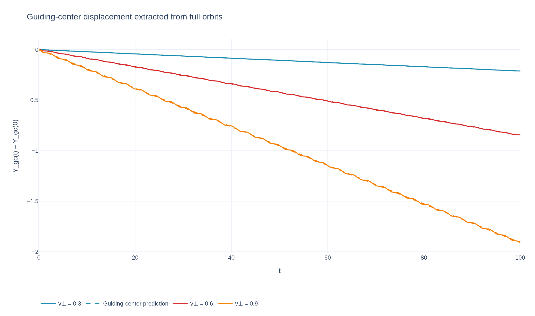
Physical problem
Gyration in a magnetic-field gradient
PDEs solved by model:
Vlasov equation:
Simulation geometry
Domain used in this run
The actual Cuboid geometry reconstructed from this run's metadata. Switch between the 3D view and physical-coordinate slices.
Domain
Cuboid
Mapping
Loading Cuboid…
Parameters
| Parameter | Value | Description |
|---|---|---|
| Loading parameters… | ||
Performance
Profiling
Struphy's built-in scope-profiler instruments every propagator, pusher and solver call — these are the real per-call timings from the run above.
Durations
Gantt (rank 0)
Region statistics
| Region | Count | Avg (s) | Min (s) | Max (s) | Total (s) |
|---|
Complete source
Simulation script
Requires Struphy with compiled kernels and Plotly. Run struphy compile once, then execute python grad-b-drift.py.
"""Grad-B drift of full-orbit test ions in a straight, nonuniform magnetic field.

B = [1 + 0.3 sin(2*pi*x/40)] e_z is divergence-free and periodic. Its field
lines are straight, so there is no curvature drift. Three positive ions with
different perpendicular speeds drift in y, with the leading guiding-center
prediction v_d = v_perp**2 B'(x_gc)/(2 B(x_gc)**2), in units q/m = 1.
The guiding-center approximation has finite-Larmor-radius corrections; only
the full-orbit speed is an exact invariant in this benchmark. Run on one rank
because this example needs the complete trajectories of individually tracked markers.

Reference: https://farside.ph.utexas.edu/teaching/plasma/lectures/node19.html
Requires the pinned Struphy with compiled kernels (`struphy compile`).
"""

import numpy as np

from struphy import (
    BoundaryParameters, DerhamOptions, EnvironmentOptions, LoadingParameters,
    SavingParameters, Simulation, Time, domains, equils, grids, maxwellians,
)
from struphy.models import Vlasov

stem = "grad-b-drift"
box, ripple = 40.0, 0.3
speeds = (0.3, 0.6, 0.9)


class PeriodicMagneticSlab(equils.HomogenSlab):
    """Externally prescribed straight magnetic field, with transverse variation."""

    def __init__(self, length=40.0, ripple=0.3):
        super().__init__(B0z=1.0, n0=1.0)
        self.params.update(length=length, ripple=ripple)

    def b_xyz(self, x, y, z):
        return 0.0 * x, 0.0 * x, 1.0 + self.params["ripple"] * np.sin(2 * np.pi * x / self.params["length"])

    def gradB_xyz(self, x, y, z):
        gradient = self.params["ripple"] * 2 * np.pi / self.params["length"] * np.cos(2 * np.pi * x / self.params["length"])
        return gradient, 0.0 * x, 0.0 * x

    def j_xyz(self, x, y, z):
        return 0.0 * x, -self.gradB_xyz(x, y, z)[0], 0.0 * x


equil = PeriodicMagneticSlab(length=box, ripple=ripple)
model = Vlasov(charge_number=1, mass_number=1.0)
model.kinetic_ions.var.add_background(maxwellians.Maxwellian3D())
markers = tuple((0.5, 0.5, 0.5, speed, 0.0, 0.0) for speed in speeds)
model.kinetic_ions.set_markers(
    loading_params=LoadingParameters(Np=len(markers), seed=7, specific_markers=markers),
    saving_params=SavingParameters(n_markers=len(markers)),
    boundary_params=BoundaryParameters(),
)
domain = domains.Cuboid(r1=box, r2=box, r3=box)
grid = grids.TensorProductGrid(num_elements=(64, 1, 1))
derham_opts = DerhamOptions(degree=(3, 1, 1))
time_opts = Time(dt=0.05, Tend=100.0, split_algo="Strang")
sim = Simulation(
    model=model, name="Grad-B drift of charged particles",
    description=(
        "Charged particles gyrate more tightly on the stronger-field side of an orbit, "
        "producing a drift perpendicular to both the magnetic field and its gradient. "
        "Three test ions demonstrate how the drift grows with perpendicular kinetic energy. "
        "The magnetic field is externally prescribed; its straight field lines exclude curvature drift."
        r" Here $$\mathbf{B}(x)=[1+0.3\sin(2\pi x/40)]\mathbf{e}_z,$$"
        r" and the ions start at :math:`(20,20,20)` with :math:`\mathbf{v}_0=(v_\perp,0,0)`,"
        r" :math:`v_\perp\in\{0.3,0.6,0.9\}` and :math:`q/m=1`. "
        r" Their measured drift is compared with the guiding-center approximation :math:`v_{\nabla B,y}=v_\perp^2 B'/(2B^2)`."
    ),
    env=EnvironmentOptions(out_folders="struphy_gallery_runs", sim_folder="grad_b_drift"),
    time_opts=time_opts, domain=domain, grid=grid, derham_opts=derham_opts, equil=equil,
)


if __name__ == "__main__":
    import plotly.graph_objects as go
    from plotly.subplots import make_subplots
    from _gallery import export_profiling, merge_metadata, save_extra_figure, save_figure

    output = sim.run(profiling_activated=True)
    # Post-processing otherwise tries to reconstruct this script-local class
    # from Struphy's built-in equilibrium catalogue. Reuse the actual object.
    output.equil = equil
    output.pproc()
    orbits = output.evaluate("kinetic_ions")
    times = orbits.t.values
    x, y, vx, vy = (orbits.sel(quantity=name).values for name in ("x", "y", "v1", "v2"))
    # The time loop can write one final step just beyond Tend because of floating-point
    # accumulation. That is complete output, as long as it reaches the requested end time.
    complete = times[-1] >= time_opts.Tend - 1e-10
    if not all(np.isfinite(a).all() for a in (x, y, vx, vy)) or not complete:
        raise RuntimeError("Incomplete or non-finite particle tracks; run this example on one MPI rank")
    if x.shape[1] != len(speeds) or np.max(np.abs(x - box / 2)) > 3 or np.max(np.abs(y - box / 2)) > 6:
        raise RuntimeError("A particle was lost or left the expected orbit region")
    speed = np.hypot(vx, vy)
    speed_drift = float(np.max(np.abs(speed / speed[0] - 1.0)))
    local_b = 1 + ripple * np.sin(2 * np.pi * x / box)
    # Remove the leading gyration before measuring the slow drift. This is an
    # approximate guiding-center coordinate, not a separate guiding-center run.
    center_y = y - vx / local_b
    measured = np.polyfit(times, center_y, 1)[0]
    gradient = -ripple * 2 * np.pi / box  # at x_gc = box/2, B = 1
    reference = 0.5 * speed[0]**2 * gradient
    drift_error = float(np.max(np.abs(measured / reference - 1.0)))
    if speed_drift > 1e-8 or drift_error > 0.08:
        raise RuntimeError(f"Grad-B benchmark failed: speed drift={speed_drift:.3g}, drift-rate error={drift_error:.3g}")

    palette = ("#168aad", "#d62828", "#f77f00")
    figure = make_subplots(rows=1, cols=2, horizontal_spacing=0.14,
                           subplot_titles=("Gyration plus a slow transverse drift", "Drift grows with perpendicular energy"))
    for j, color in enumerate(palette):
        figure.add_scatter(x=x[:, j], y=y[:, j], name=f"v⊥ = {speed[0, j]:.1f}",
                           line={"color": color, "width": 1.5}, row=1, col=1)
        figure.add_scatter(x=[speed[0, j]**2], y=[measured[j]], mode="markers", showlegend=False,
                           marker={"color": color, "size": 11}, row=1, col=2)
    square_speed = np.linspace(0, 1, 100)
    figure.add_scatter(x=square_speed, y=0.5 * square_speed * gradient, name="Guiding-center prediction",
                       line={"color": "#222", "dash": "dash"}, row=1, col=2)
    figure.update_xaxes(title_text="x", row=1, col=1)
    figure.update_yaxes(title_text="y", scaleanchor="x", scaleratio=1, row=1, col=1)
    figure.update_xaxes(title_text="v⊥²", row=1, col=2)
    figure.update_yaxes(title_text="mean drift velocity in y", row=1, col=2)
    figure.update_layout(title="Grad-B drift in a straight magnetic field", template="plotly_white",
                         legend={"orientation": "h", "y": -0.2}, margin={"l": 70, "r": 35, "t": 100, "b": 120})
    save_figure(figure, stem, height=650)
    drift = go.Figure()
    for j, color in enumerate(palette):
        drift.add_scatter(x=times, y=center_y[:, j] - center_y[0, j], name=f"v⊥ = {speed[0, j]:.1f}", line={"color": color})
        drift.add_scatter(x=times, y=reference[j] * times, name="Guiding-center prediction", showlegend=j == 0,
                          line={"color": color, "dash": "dash"})
    drift.update_layout(title="Guiding-center displacement extracted from full orbits", template="plotly_white",
                         xaxis_title="t", yaxis_title="Y_gc(t) − Y_gc(0)",
                         legend={"orientation": "h", "y": -0.2}, margin={"l": 80, "r": 30, "t": 80, "b": 110})
    figures = [save_extra_figure(drift, stem, "drift", alt="Approximate guiding centers drifting steadily across the magnetic field",
                                caption="Subtracting the leading gyration reveals the slow drift. Small oscillations remain because the guiding-center formula neglects finite-Larmor-radius corrections.")]
    merge_metadata(stem, measuredDriftVelocities=measured.tolist(), guidingCenterDriftVelocities=reference.tolist(),
                   maxDriftRateError=drift_error, maxSpeedDrift=speed_drift, figures=figures, **export_profiling(sim, stem))
See the post-processing guide for more ways to inspect the result.