Vlasov · Particle orbits
Gyromotion in a uniform magnetic field
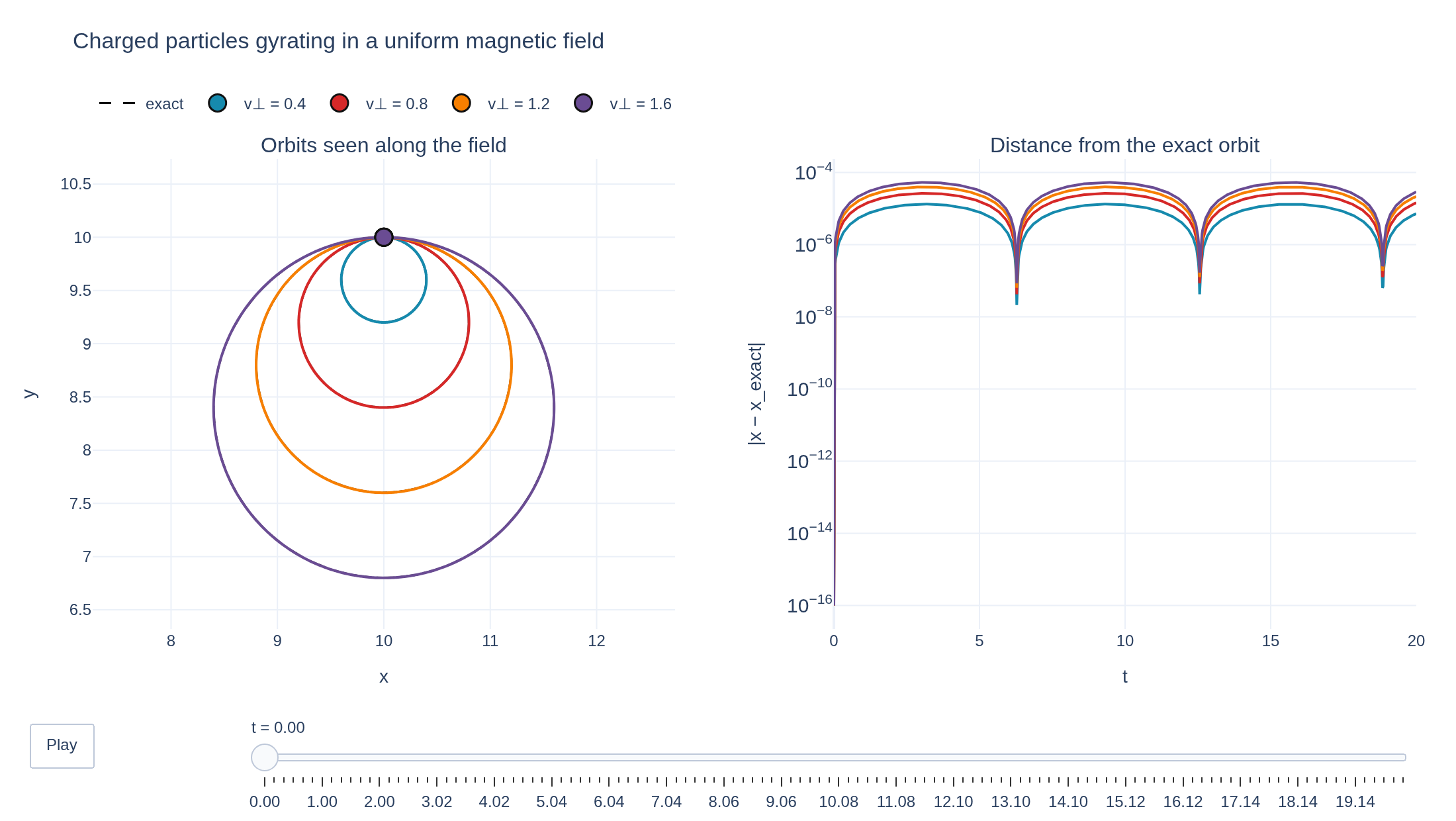
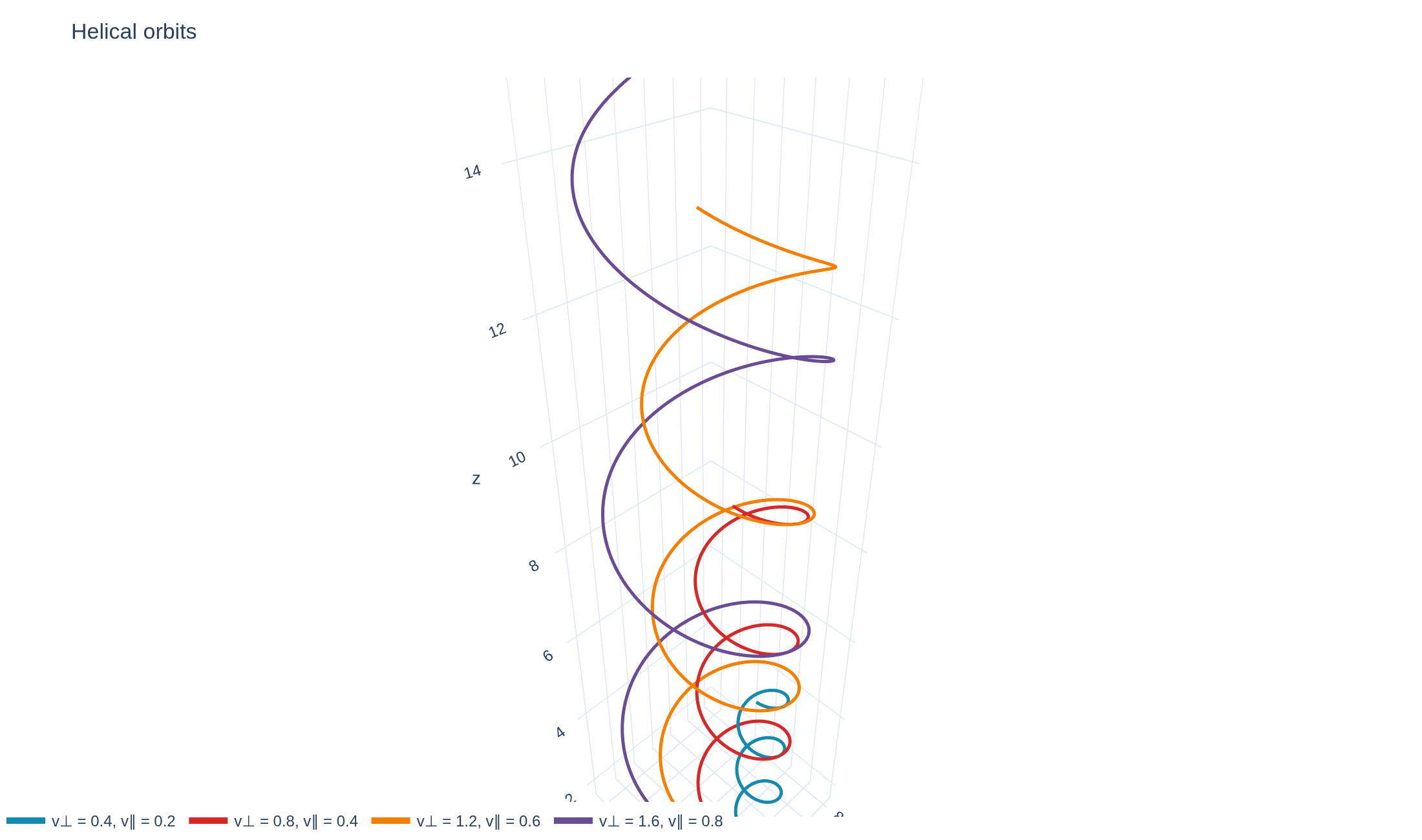
Test particles with different perpendicular speeds circle a uniform magnetic field at the same gyrofrequency, on circles whose Larmor radius grows with the perpendicular speed, while they stream freely along the field. Struphy's full-orbit pusher is compared with the exact helices.
Loading interactive figure…
Loading interactive figure…
Loading interactive figure…
Physical problem
Circles in a uniform field
PDEs solved by model:
Vlasov equation:
Simulation geometry
Domain used in this run
The actual Cuboid geometry reconstructed from this run's metadata. Switch between the 3D view and physical-coordinate slices.
Domain
Cuboid
Mapping
Loading Cuboid…
Parameters
| Parameter | Value | Description |
|---|---|---|
| Loading parameters… | ||
Performance
Profiling
Struphy's built-in scope-profiler instruments every propagator, pusher and solver call — these are the real per-call timings from the run above.
Durations
Gantt (rank 0)
Region statistics
| Region | Count | Avg (s) | Min (s) | Max (s) | Total (s) |
|---|
Complete source
Simulation script
Requires Struphy with compiled kernels and Plotly. Run struphy compile once, then execute python gyromotion.py.
"""Gyromotion of charged test particles in a uniform magnetic field, with Struphy's Vlasov model.

A particle of charge q and mass m in a uniform field B0 e_z circles the field line at the gyrofrequency
Omega = q B0 / m, on a circle of radius v_perp / Omega (the Larmor radius), and streams freely along the field.
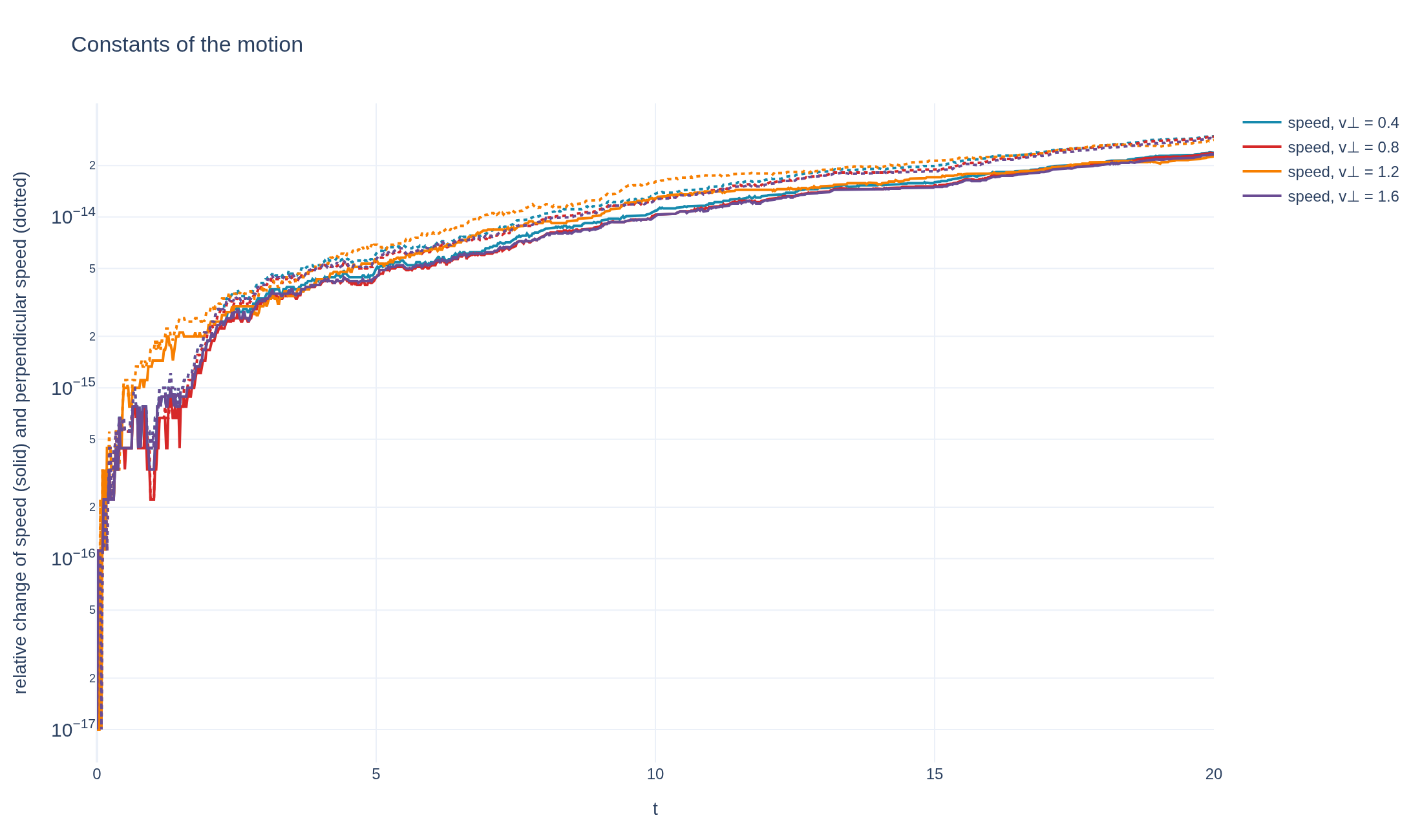
The orbit is a helix, and since a magnetic field does no work, the speed and the perpendicular speed are
constants of the motion. Four markers with different perpendicular speeds are followed and compared with the exact
helices: the gyroperiod is the same for all of them, the Larmor radius grows in proportion to v_perp.

Requires Struphy 3.3 with compiled kernels (`struphy compile`).
"""

import numpy as np
import plotly.graph_objects as go

from struphy import DerhamOptions, EnvironmentOptions, Simulation, Time, domains, equils, grids
from struphy.kinetic_background import maxwellians
from struphy.models import Vlasov
from struphy.pic.base import BoundaryParameters, LoadingParameters, SavingParameters

B0 = 1.0  # q = m = 1, so the gyrofrequency is B0
gyrofrequency = B0
box = 20.0
v_perp = (0.4, 0.8, 1.2, 1.6)
v_parallel = (0.2, 0.4, 0.6, 0.8)
centre = 0.5 * box
# About three gyroperiods. Strang splitting of the position and velocity pushes makes the orbit second order in dt; the
# default Lie-Trotter splitting is first order and leaves an error of about v * dt / 2 in the position.
time_opts = Time(dt=0.02, Tend=20.0, split_algo="Strang")

model = Vlasov(charge_number=1, mass_number=1.0)
model.kinetic_ions.var.add_background(maxwellians.Maxwellian3D())
# Every marker starts at the middle of the box with velocity (v_perp, 0, v_parallel).
markers = tuple((0.5, 0.5, 0.1, vp, 0.0, vz) for vp, vz in zip(v_perp, v_parallel))
model.kinetic_ions.set_markers(
    loading_params=LoadingParameters(Np=len(markers), seed=7, specific_markers=markers),
    saving_params=SavingParameters(n_markers=len(markers)),
    boundary_params=BoundaryParameters(),
)

sim = Simulation(
    model=model,
    name="Gyromotion in a uniform magnetic field",
    description=(
        "Test particles with different perpendicular speeds circle a uniform magnetic field at the same gyrofrequency, "
        "on circles whose Larmor radius grows with the perpendicular speed, while they stream freely along the field. "
        "Struphy's full-orbit pusher is compared with the exact helices."
    ),
    env=EnvironmentOptions(out_folders="struphy_gallery_runs", sim_folder="gyromotion"),
    time_opts=time_opts,
    domain=domains.Cuboid(r1=box, r2=box, r3=box),
    equil=equils.HomogenSlab(B0z=B0, n0=1.0),
    grid=grids.TensorProductGrid(num_elements=(4, 4, 4)),
    derham_opts=DerhamOptions(degree=(1, 1, 1)),
)


def exact_orbit(t, vp, vz, z0):
    """The helix of a marker starting at the box centre with velocity (vp, 0, vz): (x, y, z)."""
    phase = gyrofrequency * t
    radius = vp / gyrofrequency
    return centre + radius * np.sin(phase), centre + radius * (np.cos(phase) - 1.0), z0 + vz * t


if __name__ == "__main__":
    from plotly.subplots import make_subplots

    from _gallery import export_profiling, merge_metadata, save_extra_figure, save_figure

    output = sim.run(profiling_activated=True)
    output.pproc()

    # (time, marker, [x, y, z, v1, v2, v3, weight, id]), physical coordinates.
    orbits = np.asarray(output.orbits.kinetic_ions)
    n_markers = orbits.shape[1]
    times = np.arange(orbits.shape[0]) * time_opts.Tend / (orbits.shape[0] - 1)
    z0 = float(orbits[0, 0, 2])

    position_error = np.zeros((orbits.shape[0], n_markers))
    speed_drift = np.zeros_like(position_error)
    perpendicular_drift = np.zeros_like(position_error)
    radius = np.zeros(n_markers)
    exact = []
    for p in range(n_markers):
        x, y, z = exact_orbit(times, v_perp[p], v_parallel[p], z0)
        exact.append((x, y, z))
        position_error[:, p] = np.sqrt((orbits[:, p, 0] - x) ** 2 + (orbits[:, p, 1] - y) ** 2 + (orbits[:, p, 2] - z) ** 2)
        speed = np.linalg.norm(orbits[:, p, 3:6], axis=1)
        speed_drift[:, p] = np.abs(speed / speed[0] - 1.0)
        perp = np.hypot(orbits[:, p, 3], orbits[:, p, 4])
        perpendicular_drift[:, p] = np.abs(perp / perp[0] - 1.0)
        # The Larmor radius from the extent of the orbit in the plane.
        radius[p] = 0.5 * (np.ptp(orbits[:, p, 0]) + np.ptp(orbits[:, p, 1])) / 2.0
    # The measured gyrofrequency: the phase of the velocity vector v1 - i v2 = v_perp exp(i Omega t) unwrapped.
    phases = np.unwrap(np.angle(orbits[:, 0, 3] - 1j * orbits[:, 0, 4]))
    measured_frequency = float(np.polyfit(times, phases, 1)[0])
    if not (np.isfinite(position_error).all() and np.isfinite(measured_frequency)):
        raise RuntimeError("Non-finite orbits")
    print(f"gyrofrequency {measured_frequency:.5f} (exact {gyrofrequency:.5f}); "
          f"max position error {position_error.max():.2e}; max speed drift {speed_drift.max():.2e}")
    print("Larmor radii", np.round(radius, 4), "exact", np.round(np.asarray(v_perp) / gyrofrequency, 4))

    palette = ["#168aad", "#d62828", "#f77f00", "#6a4c93"]
    figure = make_subplots(rows=1, cols=2, column_widths=[0.5, 0.5], horizontal_spacing=0.12,
                           subplot_titles=("Orbits seen along the field", "Distance from the exact orbit"))
    for p in range(n_markers):
        figure.add_trace(go.Scatter(x=exact[p][0], y=exact[p][1], mode="lines", showlegend=(p == 0), name="exact",
                                    line={"color": "#111", "width": 1.5, "dash": "dash"}), row=1, col=1)
    for p in range(n_markers):
        figure.add_trace(go.Scatter(x=orbits[:, p, 0], y=orbits[:, p, 1], mode="lines", showlegend=False,
                                    line={"color": palette[p], "width": 2, "shape": "spline"}), row=1, col=1)
    head_start = len(figure.data)
    for p in range(n_markers):
        figure.add_trace(go.Scatter(x=[orbits[0, p, 0]], y=[orbits[0, p, 1]], mode="markers",
                                    name=f"v⊥ = {v_perp[p]}", marker={"color": palette[p], "size": 13,
                                                                      "line": {"color": "#111", "width": 1.5}}),
                         row=1, col=1)
    for p in range(n_markers):
        figure.add_trace(go.Scatter(x=times, y=np.maximum(position_error[:, p], 1e-16), mode="lines", showlegend=False,
                                    line={"color": palette[p], "width": 2}), row=1, col=2)

    picks = np.unique(np.linspace(0, len(times) - 1, min(120, len(times)), dtype=int))
    figure.frames = [
        go.Frame(name=f"{times[i]:.2f}", traces=list(range(head_start, head_start + n_markers)),
                 data=[go.Scatter(x=[orbits[i, p, 0]], y=[orbits[i, p, 1]]) for p in range(n_markers)])
        for i in picks
    ]
    figure.update_layout(
        title="Charged particles gyrating in a uniform magnetic field", template="plotly_white",
        margin={"l": 70, "r": 30, "t": 120, "b": 140}, title_y=0.96, legend={"orientation": "h", "y": 1.16},
        updatemenus=[{"type": "buttons", "showactive": False, "x": 0, "y": -0.2,
                      "buttons": [{"label": "Play", "method": "animate", "args": [None, {"frame": {"duration": 50, "redraw": False}, "transition": {"duration": 0}, "fromcurrent": True}]}]}],
        sliders=[{"active": 0, "x": 0.12, "len": 0.88, "y": -0.12, "currentvalue": {"prefix": "t = "},
                  "steps": [{"args": [[frame.name], {"frame": {"duration": 0, "redraw": False}, "transition": {"duration": 0}, "mode": "immediate"}], "label": frame.name, "method": "animate"} for frame in figure.frames]}],
    )
    span = 1.15 * max(v_perp)
    figure.update_xaxes(title_text="x", range=[centre - span, centre + 1.15 * max(v_perp)], row=1, col=1)
    figure.update_yaxes(title_text="y", range=[centre - 2 * span, centre + 0.4 * span], scaleanchor="x", row=1, col=1)
    figure.update_xaxes(title_text="t", row=1, col=2)
    figure.update_yaxes(title_text="|x − x_exact|", type="log", row=1, col=2)
    save_figure(figure, "gyromotion", width=1100, height=620)

    helix = go.Figure()
    for p in range(n_markers):
        helix.add_trace(go.Scatter3d(x=orbits[:, p, 0], y=orbits[:, p, 1], z=orbits[:, p, 2], mode="lines",
                                     name=f"v⊥ = {v_perp[p]}, v∥ = {v_parallel[p]}",
                                     line={"width": 5, "color": palette[p]}))
    helix.update_layout(
        title="Helical orbits", template="plotly_white", autosize=True, margin={"l": 0, "r": 0, "t": 60, "b": 0},
        scene={"xaxis_title": "x", "yaxis_title": "y", "zaxis_title": "z", "aspectmode": "data"},
        legend={"orientation": "h", "y": 0.02},
    )
    conservation = go.Figure()
    for p in range(n_markers):
        conservation.add_scatter(x=times, y=np.maximum(speed_drift[:, p], 1e-17), mode="lines", name=f"speed, v⊥ = {v_perp[p]}",
                                 line={"color": palette[p], "width": 2})
        conservation.add_scatter(x=times, y=np.maximum(perpendicular_drift[:, p], 1e-17), mode="lines", showlegend=False,
                                 line={"color": palette[p], "width": 2, "dash": "dot"})
    conservation.update_layout(
        title="Constants of the motion", template="plotly_white", autosize=True,
        xaxis_title="t", yaxis_title="relative change of speed (solid) and perpendicular speed (dotted)", yaxis_type="log",
        margin={"l": 75, "r": 30, "t": 80, "b": 60},
    )
    figures = [
        save_extra_figure(helix, "gyromotion", "helices",
                          alt="Helical orbits of four charged particles around a uniform magnetic field",
                          caption="The same four orbits in three dimensions: circles in the plane perpendicular to B, stretched "
                                  "into helices by the free streaming along the field."),
        save_extra_figure(conservation, "gyromotion", "conservation",
                          alt="Relative change of the speed and the perpendicular speed of gyrating particles",
                          caption="A magnetic field does no work, so the speed and the perpendicular speed of each marker are constant. "
                                  "The relative changes stay at round-off level."),
    ]

    merge_metadata(
        "gyromotion",
        gyrofrequency=gyrofrequency, measuredGyrofrequency=measured_frequency,
        larmorRadii={str(vp): float(r) for vp, r in zip(v_perp, radius)},
        maxPositionError=float(position_error.max()), maxSpeedDrift=float(speed_drift.max()),
        figures=figures, **export_profiling(sim, "gyromotion"),
    )
See the post-processing guide for more ways to inspect the result.