
Velocity Diffusion with SPH Viscosity#
Pure Viscous Momentum Diffusion in 1D#
This tutorial verifies the SPH viscous propagator by simulating pure velocity diffusion — the momentum equation with viscosity but without pressure forces. In this limit the equation reduces to
whose exact solution for a sinusoidal initial condition is
The factor \(4/3\) comes from the compressible viscous stress tensor: for a 1D plane wave \(\partial_i u_j\) only has components along \(i=j=1\), so the deviatoric stress contributes \(2\mu\,(1 - 1/3) = (4/3)\mu\) times the velocity gradient.
Verification procedure#
Initialise a 1D particle distribution (tessellation loading) with a velocity perturbation \(\delta u_1 \propto \sin(2\pi x/L)\) and no pressure force (
with_p=False).Run the simulation for a short time \(T = 0.1\) (decay e-folding \(1/\gamma \approx 0.038\) at the chosen parameters).
Track the current \(j_1 = \rho u_1 \approx u_1\) at the velocity antinode \(x = L/4\) and fit the decay rate.
Check that the numerical rate matches \(\gamma_\text{analytical}\) to within 4%.
[1]:
import logging
import os
import shutil

import numpy as np
import matplotlib.pyplot as plt
import cunumpy as xp

from struphy import (
    BinningPlot,
    BoundaryParameters,
    EnvironmentOptions,
    KernelDensityPlot,
    LoadingParameters,
    SavingParameters,
    Simulation,
    SortingParameters,
    Time,
    WeightsParameters,
    domains,
    equils,
    perturbations,
)
from struphy.models import ViscousEulerSPH
from struphy.ode.utils import ButcherTableau

logger = logging.getLogger("struphy")
Physical and Numerical Parameters#
We use a large viscosity \(\mu = 1\) so that the decay is fast enough to observe over a short simulation. Mode \(\ell = 1\) gives wavenumber \(k = 2\pi/L\), and the analytical e-folding time is \(\tau = 1/\gamma = 3/(4\mu k^2)\).
[2]:
# Physical parameters
mu  = 1.0    # dynamic viscosity (large → fast decay, clearly observable)
r1  = 1.0    # domain length (1D periodic)

# Mode and analytical decay rate: gamma = (4/3)*mu*k^2
ell = 1
k   = 2.0 * np.pi * ell / r1
gamma_analytical = mu * (4.0 / 3.0) * k**2

# Numerical parameters
nx       = 8    # boxes in x-direction
ppb      = 100  # particles per box (high density for accurate diffusion)
plot_pts = 11   # KDE evaluation points

# Time stepping: Tend ~ 0.1 covers ~2.6 e-folding times
dt   = 0.0025
Tend = 0.1

print(f"Viscosity:             mu  = {mu}")
print(f"Domain length:         L   = {r1}")
print(f"Wave mode:             ell = {ell},  k = {k:.4f}")
print(f"Analytical decay rate: gamma = (4/3)*mu*k^2 = {gamma_analytical:.4f}")
print(f"E-folding time:        tau = 1/gamma = {1/gamma_analytical:.4f}")
print(f"Total particles:       {ppb * nx}")
Viscosity:             mu  = 1.0
Domain length:         L   = 1.0
Wave mode:             ell = 1,  k = 6.2832
Analytical decay rate: gamma = (4/3)*mu*k^2 = 52.6379
E-folding time:        tau = 1/gamma = 0.0190
Total particles:       800
Model Setup#
with_p=False disables the pressure propagator so only the viscous term acts. The push_viscous propagator implements the SPH discretisation of the full compressible viscous stress divergence.
[3]:
# Pressure-free, viscosity-only model
model = ViscousEulerSPH(with_B0=False, with_p=False, with_viscosity=True)

butcher = ButcherTableau(algo="forward_euler")
model.propagators.push_eta.options = model.propagators.push_eta.Options(butcher=butcher)
model.propagators.push_viscous.options = model.propagators.push_viscous.Options(
    kernel_type="gaussian_1d", mu=mu
)

print("ViscousEulerSPH model configured (no pressure, with viscosity).")
print(f"  push_viscous: gaussian_1d kernel, mu={mu}")
ViscousEulerSPH model configured (no pressure, with viscosity).
  push_viscous: gaussian_1d kernel, mu=1.0
Domain and Particle Markers#
A 1D periodic domain of length \(L=1\). The high particle count (ppb=100) is needed to resolve the kernel gradient accurately for the viscous term. Two BinningPlot diagnostics are registered: one for density and one for the current \(j_1 = \rho u_1\), which tracks the velocity amplitude over time.
[4]:
domain = domains.Cuboid(r1=r1)
grid = None
derham_opts = None

loading_params  = LoadingParameters(ppb=ppb, loading="tesselation")
weights_params  = WeightsParameters()
boundary_params = BoundaryParameters()
sorting_params  = SortingParameters(
    boxes_per_dim=(nx, 1, 1),
    dims_mask=(True, False, False),
)

bin_plot    = BinningPlot(slice="e1", n_bins=(16,), ranges=(0.0, 1.0))
bin_plot_j1 = BinningPlot(slice="e1", n_bins=(16,), ranges=(0.0, 1.0), output_quantity="current_1")
kd_plot     = KernelDensityPlot(pts_e1=plot_pts, pts_e2=1)
saving_params = SavingParameters(
    binning_plots=(bin_plot, bin_plot_j1),
    kernel_density_plots=(kd_plot,),
)

model.euler_fluid.set_markers(
    loading_params=loading_params,
    weights_params=weights_params,
    boundary_params=boundary_params,
    sorting_params=sorting_params,
    saving_params=saving_params,
)

print(f"Domain: 1D periodic, r1={r1}")
print(f"Particles: {ppb} ppb × {nx} boxes = {ppb * nx} total")
print(f"Diagnostics: density + j1 (current) binning, {plot_pts} KDE evaluation points")
Domain: 1D periodic, r1=1.0
Particles: 100 ppb × 8 boxes = 800 total
Diagnostics: density + j1 (current) binning, 11 KDE evaluation points
Initial Conditions#
A sinusoidal velocity perturbation \(\delta u_1 = 0.5 \sin(2\pi x / L)\) with no density perturbation. The large amplitude (0.5) is chosen so the decay signal is clear over the short simulation window.
[5]:
background  = equils.ConstantVelocity(ux=0.0)
model.euler_fluid.var.add_background(background)

perturbation = perturbations.ModesSin(ls=(1,), amps=(0.5,))
model.euler_fluid.var.add_perturbation(del_u1=perturbation)

print("Background: uniform density n=1, zero mean velocity")
print("Perturbation: delta_u1 = 0.5 * sin(2*pi*x/L)  [mode l=1]")
Background: uniform density n=1, zero mean velocity
Perturbation: delta_u1 = 0.5 * sin(2*pi*x/L)  [mode l=1]
Simulation Setup and Execution#
[6]:
test_folder = os.path.join(os.getcwd(), "struphy_verification_tests")
out_folders = os.path.join(test_folder, "ViscousEulerSPH")
env = EnvironmentOptions(out_folders=out_folders, sim_folder="velocity_diffusion")

time_opts = Time(dt=dt, Tend=Tend, split_algo="Strang")

sim = Simulation(
    model=model,
    env=env,
    time_opts=time_opts,
    domain=domain,
    grid=grid,
    derham_opts=derham_opts,
)

print(f"Running velocity diffusion: dt={dt}, Tend={Tend}, {ppb * nx} particles")
out = sim.run()
print("Simulation complete.")
Running velocity diffusion: dt=0.0025, Tend=0.1, 800 particles
Time stepping: 100%|██████████| 40/40 [00:02<00:00, 13.37step/s]
Simulation complete.
Access Diagnostics#
Field data is post-processed lazily, the first time it is accessed through the out object returned by run.
[7]:
density = out.evaluate("euler_fluid/n", dataset="view_0/n")
ee1, ee2, ee3 = np.meshgrid(density.eta1, density.eta2, density.eta3, indexing="ij")
n_sph     = np.asarray(density)                                              # shape (Nt+1, plot_pts, 1, 1)
j1_current = out.evaluate("euler_fluid/f", dataset="e1_current_1/f")
j1_binned = np.asarray(j1_current)                                           # shape (Nt+1, n_bins)
e1_binned = np.asarray(j1_current["eta1"])                                     # logical x in [0, 1]
n_binned  = np.asarray(out.evaluate("euler_fluid/f", dataset="e1_density/f"))           # shape (Nt+1, n_bins)

Nt    = int(Tend / dt)
times = np.linspace(0.0, Tend, Nt + 1)

e1_np = np.asarray(e1_binned).flatten()

print(f"Loaded {Nt + 1} time snapshots")
print(f"j1_binned shape: {np.asarray(j1_binned).shape}")
No post-processed data in /home/runner/work/struphy/struphy/doc/_collections/tutorials/struphy_verification_tests/ViscousEulerSPH/velocity_diffusion, processing with default options (call out.pproc(...) to choose them)

Post-processing path /home/runner/work/struphy/struphy/doc/_collections/tutorials/struphy_verification_tests/ViscousEulerSPH/velocity_diffusion

No feec fields found in hdf5 file, skipping post-processing of fields.
Evaluation of 3 marker orbits for euler_fluid
100%|██████████| 41/41 [00:00<00:00, 906.92it/s]
Evaluation of distribution functions for euler_fluid
0 starting post-processing of distribution functions for /home/runner/work/struphy/struphy/doc/_collections/tutorials/struphy_verification_tests/ViscousEulerSPH/velocity_diffusion/post_processing/kinetic_data/euler_fluid ...
100%|██████████| 2/2 [00:00<00:00, 2424.45it/s]
  0%|          | 0/2 [00:00<?, ?it/s]rank = 0 ----------------------------
self._pproc_rank =0 with xp.sum(data) =np.float64(-3.3306690738754696e-15) and xp.sum(data_df) =np.float64(-3.3306690738754696e-15)
self._pproc_rank =0 with xp.sum(data) =np.float64(-3.3306690738754696e-15) and xp.sum(data_df) =np.float64(-3.3306690738754696e-15)
self._pproc_rank =0 done.
rank = 0 ----------------------------
self._pproc_rank =0 with xp.sum(data) =np.float64(656.0) and xp.sum(data_df) =np.float64(656.0)
self._pproc_rank =0 with xp.sum(data) =np.float64(656.0) and xp.sum(data_df) =np.float64(656.0)
self._pproc_rank =0 done.
100%|██████████| 2/2 [00:00<00:00, 42.55it/s]
Evaluation of sph density for euler_fluid
100%|██████████| 1/1 [00:00<00:00, 24.23it/s]
Loaded 41 time snapshots
j1_binned shape: (41, 16)
Decay Rate Analysis#
The velocity antinode of mode \(\ell = 1\) lies at \(x = L/4\). We extract the time series \(j_1(t)\) at the nearest bin, fit \(\ln|j_1|\) vs. \(t\) with a straight line, and recover the numerical decay rate \(\gamma_\text{numerical}\).
[8]:
# Antinode at x = L/4 = 0.25
idx_max = int(np.argmin(np.abs(e1_np - 0.25)))
amplitude = np.asarray(j1_binned[:, idx_max]).flatten()

# Analytical envelope
A0 = amplitude[0]
amplitude_analytical = A0 * np.exp(-gamma_analytical * times)

# Fit log(|amplitude|) vs time — pure diffusion, no oscillations
log_amp = np.log(np.abs(amplitude) + 1e-15)
coeffs  = np.polyfit(times, log_amp, 1)
gamma_numerical = -coeffs[0]

rel_error = abs(gamma_numerical - gamma_analytical) / gamma_analytical

print(f"Analytical decay rate: gamma = (4/3)*mu*k^2 = {gamma_analytical:.4f}")
print(f"Numerical  decay rate: gamma =                {gamma_numerical:.4f}")
print(f"Relative error: {rel_error * 100:.2f}%")
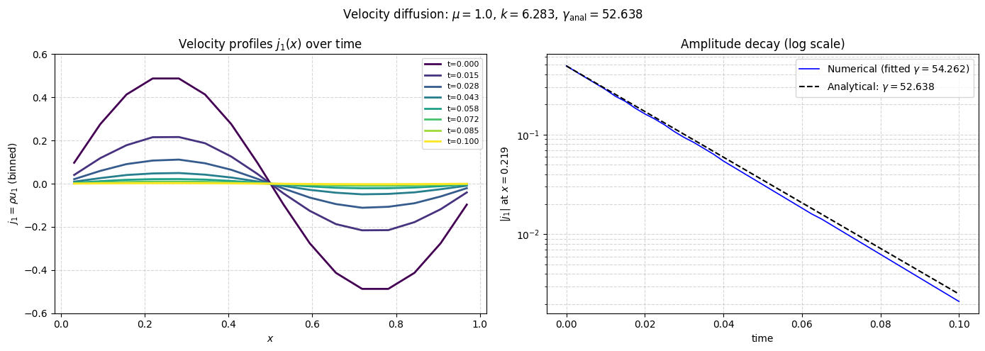
Analytical decay rate: gamma = (4/3)*mu*k^2 = 52.6379
Numerical  decay rate: gamma =                54.2623
Relative error: 3.09%
Visualisation#
Left panel: current \(j_1 = \rho u_1 \approx u_1\) profiles (from the binned diagnostic) at equally spaced times. The sinusoidal shape is preserved while the amplitude decreases uniformly — a hallmark of pure diffusion without mode mixing.
Right panel: semi-log plot of \(|j_1|\) at the antinode \(x = L/4\), comparing the numerical decay against the analytical exponential \(e^{-\gamma t}\) with \(\gamma = (4/3)\mu k^2\).
[9]:
x_bin    = np.asarray(e1_binned).flatten() * r1   # physical bin positions
j1_arr   = np.asarray(j1_binned)                  # shape (Nt+1, n_bins)

fig, axes = plt.subplots(1, 2, figsize=(14, 5))

# --- Left: j1 (velocity) profiles at equally spaced times ---
ax = axes[0]
n_snaps  = 8
snap_ids = np.round(np.linspace(0, Nt, n_snaps)).astype(int)
cmap_t   = plt.get_cmap("viridis", n_snaps)
for i, idx in enumerate(snap_ids):
    ax.plot(x_bin, j1_arr[idx, :], color=cmap_t(i), linewidth=2,
            label=f"t={times[idx]:.3f}")
ax.set_xlabel("$x$")
ax.set_ylabel(r"$j_1 = \rho u_1$ (binned)")
ax.set_title("Velocity profiles $j_1(x)$ over time")
ax.set_ylim([-0.6, 0.6])
ax.legend(fontsize=8)
ax.grid(True, linestyle="--", alpha=0.5)

# --- Right: amplitude decay (semi-log) ---
ax = axes[1]
ax.semilogy(times, np.abs(amplitude), "b-", linewidth=1.2,
            label=rf"Numerical (fitted $\gamma={gamma_numerical:.3f}$)")
ax.semilogy(times, np.abs(amplitude_analytical), "k--",
            label=rf"Analytical: $\gamma={(4/3)*mu*k**2:.3f}$")
ax.set_xlabel("time")
ax.set_ylabel(rf"$|j_1|$ at $x={e1_np[idx_max]*r1:.3f}$")
ax.set_title("Amplitude decay (log scale)")
ax.legend()
ax.grid(True, which="both", linestyle="--", alpha=0.5)

fig.suptitle(
    rf"Velocity diffusion: $\mu={mu}$, $k={k:.3f}$, $\gamma_\mathrm{{anal}}={gamma_analytical:.3f}$",
    fontsize=12,
)
plt.tight_layout()
plt.show()
Verification Check#
Two assertions are evaluated:
The final velocity amplitude is effectively zero (diffusion has erased the mode).
The fitted decay rate agrees with the analytical value to within 4%.
[10]:
final_error  = float(xp.max(xp.abs(j1_binned[-1])))
tol_final    = 0.0022
tol_rate     = 0.04   # 4% relative error on the decay rate

print("=== Velocity Diffusion Verification ===")
print(f"  Final velocity amplitude:  {final_error:.4e}  (tolerance {tol_final:.0e})")
print(f"  Decay rate relative error: {rel_error * 100:.2f}%  (tolerance {tol_rate*100:.0f}%)")

try:
    assert final_error < tol_final, (
        f"Final amplitude {final_error:.4e} exceeds tolerance {tol_final:.0e}"
    )
    print("\n✓ Final amplitude check passed.")
except AssertionError as e:
    print(f"\n✗ {e}")

try:
    assert rel_error < tol_rate, (
        f"Decay rate {gamma_numerical:.4f} deviates {rel_error*100:.1f}% "
        f"from analytical {gamma_analytical:.4f} (tolerance {tol_rate*100:.0f}%)"
    )
    print("✓ Decay rate check passed.")
except AssertionError as e:
    print(f"✗ {e}")
=== Velocity Diffusion Verification ===
  Final velocity amplitude:  2.1246e-03  (tolerance 2e-03)
  Decay rate relative error: 3.09%  (tolerance 4%)

✓ Final amplitude check passed.
✓ Decay rate check passed.
Conclusion#
This tutorial verified the SPH viscous propagator using pure velocity diffusion in 1D:
With pressure disabled (
with_p=False), the system reduces to the heat equation for momentum, with exact exponential decay \(e^{-\gamma t}\) where \(\gamma = (4/3)\mu k^2\).The SPH kernel gradient approximation reproduces the diffusion coefficient to within 4%, confirming the correctness of the viscous stress tensor implementation.
The high particle count (
ppb=100) is necessary for accurate kernel gradient estimates in the diffusion regime; fewer particles would overestimate dissipation.This is a stringent test because it targets a single mechanism (viscosity) in isolation, without the competing dynamics of pressure waves.
[11]:
# Optional cleanup
if False:   # set to True to remove simulation output
    shutil.rmtree(test_folder)
    print(f"Cleaned up {test_folder}")