ColdPlasma · Electromagnetic waves
Cold-plasma oscillation
A cosine electric field along the magnetic field displaces a cold electron fluid, which oscillates at the plasma frequency. The field and flow energies trade places as cos² and sin² of the frequency, and the measured frequency follows the square root of the density.
Loading interactive figure…
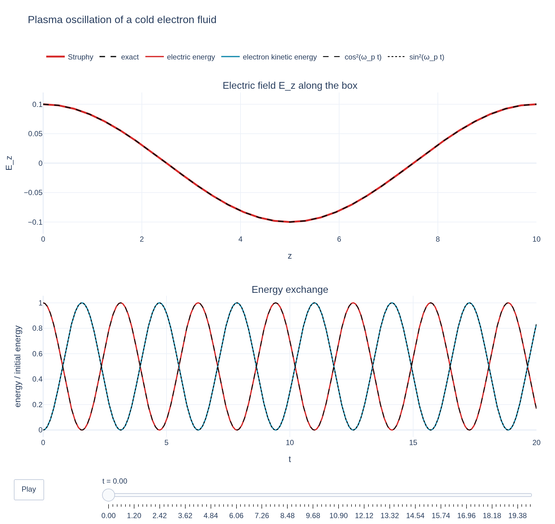
Loading interactive figure…
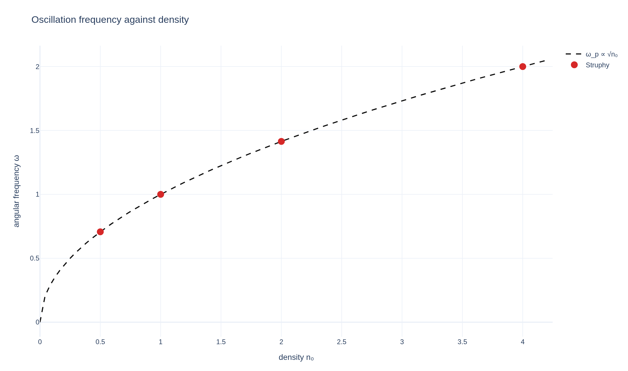
Physical problem
A cold plasma rings at its plasma frequency
PDEs solved by model:
Cold-plasma current:
Faraday's law:
Ampère's law:
where denotes an inhomogeneous background.
Simulation geometry
Domain used in this run
The actual Cuboid geometry reconstructed from this run's metadata. Switch between the 3D view and physical-coordinate slices.
Domain
Cuboid
Mapping
Loading Cuboid…
Parameters
| Parameter | Value | Description |
|---|---|---|
| Loading parameters… | ||
Performance
Profiling
Struphy's built-in scope-profiler instruments every propagator, pusher and solver call — these are the real per-call timings from the run above.
Durations
Gantt (rank 0)
Region statistics
| Region | Count | Avg (s) | Min (s) | Max (s) | Total (s) |
|---|
Complete source
Simulation script
Requires Struphy with compiled kernels and Plotly. Run struphy compile once, then execute python cold-plasma-oscillation.py.
"""Plasma oscillation of a cold electron fluid, with Struphy's ColdPlasma model.

A long-wavelength electric field E_z(z) = a cos(k z), parallel to the magnetic field and to its own
wavevector, pushes the electrons against the ions. The charge separation pulls them back, and the cold plasma
oscillates at the plasma frequency omega_p, independently of k and of the background field, with nothing to damp it.
Its energy passes back and forth between the electric field and the electron flow, as cos^2(omega_p t) and
sin^2(omega_p t). The plasma frequency scales as sqrt(n0), which a short scan over the density confirms.

Requires Struphy 3.3 with compiled kernels (`struphy compile`).
"""

import numpy as np
import plotly.graph_objects as go

from struphy import DerhamOptions, EnvironmentOptions, Simulation, Time, domains, equils, grids, perturbations
from struphy.models import ColdPlasma

# Time in units of the inverse cyclotron frequency and alpha = omega_p / omega_c = 1: at n0 = 1 the plasma
# frequency is 1 (as in the cold-plasma-waves example).
alpha, epsilon = 1.0, 1.0
length = 10.0  # box length along z
amplitude = 0.1
densities = (0.5, 1.0, 2.0, 4.0)  # the scan; the example itself is the n0 = 1 run
time_opts = Time(dt=0.02, Tend=20.0)
grid = grids.TensorProductGrid(num_elements=(1, 1, 32))
derham_opts = DerhamOptions(degree=(1, 1, 3))
domain = domains.Cuboid(r3=length)


def make_simulation(n0, folder, **extra):
    """The cold-plasma model with the density n0 and one long-wavelength cosine mode in E_z."""
    model = ColdPlasma(alpha=alpha, epsilon=epsilon)
    model.propagators.maxwell.options = model.propagators.maxwell.Options(algo="implicit")
    model.em_fields.e_field.add_perturbation(
        perturbations.ModesCos(ns=(1,), amps=(amplitude,), comp=2, Lz=length, given_in_basis="physical")
    )
    return Simulation(
        model=model,
        env=EnvironmentOptions(out_folders="struphy_gallery_runs", sim_folder=folder),
        time_opts=time_opts,
        domain=domain,
        equil=equils.HomogenSlab(B0x=0.0, B0y=0.0, B0z=1.0, n0=n0),
        grid=grid,
        derham_opts=derham_opts,
        **extra,
    )


sim = make_simulation(
    1.0,
    "cold_plasma_oscillation",
    name="Cold-plasma oscillation",
    description=(
        "A cosine electric field along the magnetic field displaces a cold electron fluid, which oscillates "
        "at the plasma frequency. The field and flow energies trade places as cos² and sin² of the frequency, "
        "and the measured frequency follows the square root of the density."
    ),
)


def mode_amplitude(run):
    """Time, and the amplitude of the cos(k z) mode of E_z, from a post-processed run."""
    e_z = run.evaluate("em_fields/e_field_xyz").isel(e1=0, e2=0, component=2)
    z = e_z.e3.values
    return e_z.t.values, 2.0 * np.mean(e_z.values * np.cos(2.0 * np.pi * z), axis=1)


def oscillation_frequency(times, values):
    """The angular frequency from the zero crossings of an oscillating signal, interpolated linearly."""
    crossings = np.where(np.diff(np.sign(values)) != 0)[0]
    roots = times[crossings] - values[crossings] * (times[crossings + 1] - times[crossings]) / (
        values[crossings + 1] - values[crossings]
    )
    return float(np.pi / np.mean(np.diff(roots)))


if __name__ == "__main__":
    from plotly.subplots import make_subplots

    from _gallery import export_profiling, is_root, merge_metadata, save_extra_figure, save_figure

    runs = {1.0: sim.run(profiling_activated=True)}
    for n0 in densities:
        if n0 != 1.0:
            runs[n0] = make_simulation(n0, f"cold_plasma_oscillation_n{n0}").run()
    for run in runs.values():
        run.pproc(physical=True)

    measured = {}
    for n0, run in runs.items():
        times, values = mode_amplitude(run)
        measured[n0] = oscillation_frequency(times, values)
    exact = {n0: alpha / epsilon * np.sqrt(n0) for n0 in runs}
    if not all(np.isfinite(list(measured.values()))):
        raise RuntimeError("A plasma frequency could not be measured")
    if is_root():
        for n0 in runs:
            print(f"n0 = {n0}: omega = {measured[n0]:.4f} (omega_p = {exact[n0]:.4f})")

    run = runs[1.0]
    omega_p = exact[1.0]
    times, values = mode_amplitude(run)
    e_z = run.evaluate("em_fields/e_field_xyz").isel(e1=0, e2=0, component=2)
    z = e_z.e3.values * length
    electric = np.asarray(run.scalars["electric_energy"])
    kinetic = np.asarray(run.scalars["kinetic_energy"])
    scalar_times = np.asarray(run.time)[: len(electric)]
    total = np.asarray(run.scalars["total_energy"])
    energy_scale = float(total[0])

    def profile_traces(index):
        return [
            go.Scatter(x=z, y=e_z.values[index], mode="lines", name="Struphy",
                       line={"color": "#d62828", "width": 3}),
            go.Scatter(x=z, y=amplitude * np.cos(omega_p * times[index]) * np.cos(2 * np.pi * z / length),
                       mode="lines", name="exact", line={"color": "#111", "width": 2, "dash": "dash"}),
        ]

    picks = np.unique(np.linspace(0, len(times) - 1, min(100, len(times)), dtype=int))
    figure = make_subplots(rows=2, cols=1, vertical_spacing=0.18,
                           subplot_titles=("Electric field E_z along the box", "Energy exchange"))
    for trace in profile_traces(0):
        figure.add_trace(trace, row=1, col=1)
    figure.add_scatter(x=scalar_times, y=electric / energy_scale, mode="lines", name="electric energy",
                       line={"color": "#d62828", "width": 2}, row=2, col=1)
    figure.add_scatter(x=scalar_times, y=kinetic / energy_scale, mode="lines", name="electron kinetic energy",
                       line={"color": "#168aad", "width": 2}, row=2, col=1)
    figure.add_scatter(x=scalar_times, y=np.cos(omega_p * scalar_times) ** 2, mode="lines", name="cos²(ω_p t)",
                       line={"color": "#111", "width": 1.5, "dash": "dash"}, row=2, col=1)
    figure.add_scatter(x=scalar_times, y=np.sin(omega_p * scalar_times) ** 2, mode="lines", name="sin²(ω_p t)",
                       line={"color": "#111", "width": 1.5, "dash": "dot"}, row=2, col=1)
    figure.frames = [go.Frame(name=f"{times[i]:.2f}", data=profile_traces(i), traces=[0, 1]) for i in picks]
    figure.update_layout(
        title="Plasma oscillation of a cold electron fluid", template="plotly_white",
        margin={"l": 70, "r": 30, "t": 150, "b": 140}, title_y=0.97, legend={"orientation": "h", "y": 1.13},
        updatemenus=[{"type": "buttons", "showactive": False, "x": 0, "y": -0.12,
                      "buttons": [{"label": "Play", "method": "animate", "args": [None, {"frame": {"duration": 60, "redraw": False}, "transition": {"duration": 0}, "fromcurrent": True}]}]}],
        sliders=[{"active": 0, "x": 0.12, "len": 0.88, "y": -0.07, "currentvalue": {"prefix": "t = "},
                  "steps": [{"args": [[frame.name], {"frame": {"duration": 0, "redraw": False}, "transition": {"duration": 0}, "mode": "immediate"}], "label": frame.name, "method": "animate"} for frame in figure.frames]}],
    )
    figure.update_xaxes(title_text="z", range=[0, length], row=1, col=1)
    figure.update_yaxes(title_text="E_z", range=[-1.2 * amplitude, 1.2 * amplitude], row=1, col=1)
    figure.update_xaxes(title_text="t", row=2, col=1)
    figure.update_yaxes(title_text="energy / initial energy", row=2, col=1)
    save_figure(figure, "cold-plasma-oscillation", width=900, height=850)

    # The frequency against the density, on the line omega = omega_p.
    n_line = np.linspace(0.0, max(densities) * 1.05, 100)
    scan = go.Figure()
    scan.add_scatter(x=n_line, y=alpha / epsilon * np.sqrt(n_line), mode="lines", name="ω_p ∝ √n₀",
                     line={"color": "#111", "width": 2, "dash": "dash"})
    scan.add_scatter(x=list(measured), y=list(measured.values()), mode="markers", name="Struphy",
                     marker={"color": "#d62828", "size": 12})
    scan.update_layout(title="Oscillation frequency against density", template="plotly_white",
                       xaxis_title="density n₀", yaxis_title="angular frequency ω",
                       margin={"l": 70, "r": 30, "t": 80, "b": 60})
    figures = [
        save_extra_figure(
            scan, "cold-plasma-oscillation", "frequency-scan",
            alt="Measured oscillation frequency of a cold plasma against density, on the square-root law",
            caption=(
                "The oscillation frequency of the same run at four densities, measured from the zero crossings of the "
                "field, on the analytic plasma frequency ω_p = √n₀ (α = 1)."
            ),
        ),
    ]

    merge_metadata(
        "cold-plasma-oscillation",
        plasmaFrequency=omega_p,
        measuredFrequency=measured[1.0],
        frequencyScan={str(n0): {"measured": measured[n0], "exact": exact[n0]} for n0 in runs},
        figures=figures,
        **export_profiling(sim, "cold-plasma-oscillation"),
    )
See the post-processing guide for more ways to inspect the result.