ColdPlasma · Electromagnetic waves
Cold-plasma wave packets
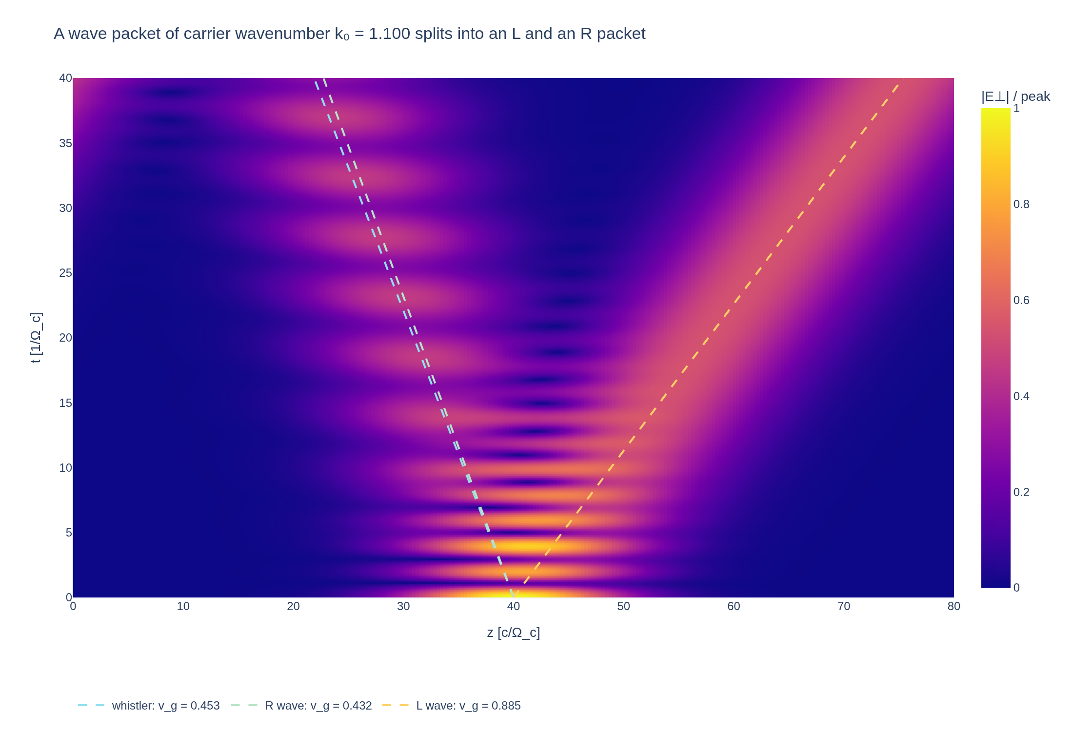
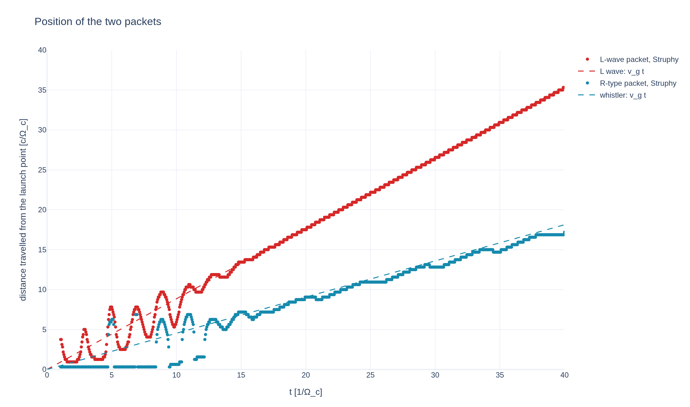
A Gaussian packet of circularly polarized electric field splits, in a magnetized cold plasma, into a fast L-wave packet and a slow, spreading R-wave packet that leave the launch point in opposite directions. Their speeds are the group velocities of the cold-plasma dispersion relation.
Loading interactive figure…
Loading interactive figure…
Physical problem
A packet splits into a fast and a slow wave
PDEs solved by model:
Cold-plasma current:
Faraday's law:
Ampère's law:
where denotes an inhomogeneous background.
Simulation geometry
Domain used in this run
The actual Cuboid geometry reconstructed from this run's metadata. Switch between the 3D view and physical-coordinate slices.
Domain
Cuboid
Mapping
Loading Cuboid…
Parameters
| Parameter | Value | Description |
|---|---|---|
| Loading parameters… | ||
Performance
Profiling
Struphy's built-in scope-profiler instruments every propagator, pusher and solver call — these are the real per-call timings from the run above.
Durations
Gantt (rank 0)
Region statistics
| Region | Count | Avg (s) | Min (s) | Max (s) | Total (s) |
|---|
Complete source
Simulation script
Requires Struphy with compiled kernels and Plotly. Run struphy compile once, then execute python cold-plasma-wave-packet.py.
"""Wave packets in a cold magnetized plasma, with Struphy's ColdPlasma model.

A cold electron fluid in a uniform field B0 e_z carries two circularly polarized waves along the field: the right-hand R wave, with its
whistler branch below the electron cyclotron frequency and an upper branch above the R cutoff, and the left-hand L wave. Their dispersion
relations differ, and so do their group velocities d omega / d k. A Gaussian packet of E_x = env cos(k0 z), E_y = -env sin(k0 z), with no
magnetic field and no current, is launched from the middle of the box. Its two circular components, e^(+i k0 z) and e^(-i k0 z), have opposite
handedness relative to their direction of propagation, so the packet splits into an L-wave packet running one way and an R-type packet running the
other way: the L packet is fast, the R packet slow and spreading, since the whistler frequency depends strongly on k. The measured speed of
each packet is compared with the analytic group velocity d omega / d k of the cold-plasma dispersion relation.

Requires Struphy 3.3 with compiled kernels (`struphy compile`).
"""

import numpy as np
import plotly.graph_objects as go

from struphy import DerhamOptions, EnvironmentOptions, Simulation, Time, domains, equils, grids
from struphy.initial.base import GenericPerturbation
from struphy.models import ColdPlasma

# Plasma frequency equal to the cyclotron frequency, time in units of the inverse cyclotron frequency, c = 1.
alpha, epsilon, n0, B0z = 1.0, 1.0, 1.0, 1.0
length = 80.0
center = 0.5 * length
mode_number = 14
k0 = 2 * np.pi * mode_number / length  # the carrier wavenumber
width = 7.0  # of the Gaussian envelope
amplitude = 0.05
time_opts = Time(dt=0.05, Tend=40.0)
grid = grids.TensorProductGrid(num_elements=(1, 1, 256))
derham_opts = DerhamOptions(degree=(1, 1, 3))
domain = domains.Cuboid(r3=length)
equil = equils.HomogenSlab(B0x=0.0, B0y=0.0, B0z=B0z, n0=n0)


def branch_frequency(k, wave):
    """Frequency of the whistler, the upper R wave or the L wave along B0, in units of the cyclotron frequency.

    With c = 1, k^2 = omega^2 - omega_p^2 omega / (omega -+ Omega_c), i.e. the cubic
    omega^3 -+ Omega_c omega^2 - (omega_p^2 + k^2) omega +- k^2 Omega_c = 0 with the upper sign for the R wave. The whistler is the
    middle positive root of the R cubic, the upper R wave its largest root, and the L wave the largest root of the L cubic.
    """
    if wave == "whistler":
        return np.sort(np.roots([1.0, -1.0, -(alpha**2 + k**2), k**2]).real)[-2]
    if wave == "R wave":
        return np.sort(np.roots([1.0, -1.0, -(alpha**2 + k**2), k**2]).real)[-1]
    return np.sort(np.roots([1.0, 1.0, -(alpha**2 + k**2), -(k**2)]).real)[-1]


def group_velocity(k, wave, step=1e-4):
    return (branch_frequency(k + step, wave) - branch_frequency(k - step, wave)) / (2 * step)


def envelope(z):
    return amplitude * np.exp(-0.5 * ((z - center) / width) ** 2)


model = ColdPlasma(alpha=alpha, epsilon=epsilon)
model.propagators.maxwell.options = model.propagators.maxwell.Options(algo="implicit")
# The carrier of the packet: E_x = env cos(k0 z), E_y = -env sin(k0 z).
model.em_fields.e_field.add_perturbation(
    GenericPerturbation(lambda x, y, z: envelope(z) * np.cos(k0 * z), given_in_basis="physical", comp=0)
)
model.em_fields.e_field.add_perturbation(
    GenericPerturbation(lambda x, y, z: -envelope(z) * np.sin(k0 * z), given_in_basis="physical", comp=1)
)

sim = Simulation(
    model=model,
    name="Cold-plasma wave packets",
    description=(
        "A Gaussian packet of circularly polarized electric field splits, in a magnetized cold plasma, into a fast L-wave packet "
        "and a slow, spreading R-wave packet that leave the launch point in opposite directions. Their speeds are the group "
        "velocities of the cold-plasma dispersion relation."
    ),
    env=EnvironmentOptions(out_folders="struphy_gallery_runs", sim_folder="cold_plasma_wave_packet"),
    time_opts=time_opts,
    domain=domain,
    equil=equil,
    grid=grid,
    derham_opts=derham_opts,
)


def packet_energy(run):
    """Time, position and the transverse electric energy density |E_perp|^2(t, z) of a post-processed run."""
    e_field = run.evaluate("em_fields/e_field_xyz").isel(e1=0, e2=0)
    density = e_field.isel(component=0).values ** 2 + e_field.isel(component=1).values ** 2
    return e_field.t.values, e_field.e3.values * length, density


if __name__ == "__main__":
    from plotly.subplots import make_subplots

    from _gallery import export_profiling, is_root, merge_metadata, save_extra_figure, save_figure

    output = sim.run(profiling_activated=True)
    output.pproc(physical=True)

    times, z, density = packet_energy(output)
    waves = ("whistler", "R wave", "L wave")
    tracked = ("whistler", "L wave")  # the slow packet holds the whistler and upper R branches, of almost equal speed
    exact_speed = {wave: group_velocity(k0, wave) for wave in waves}
    exact_frequency = {wave: branch_frequency(k0, wave) for wave in waves}

    def track_peak(side, speed):
        """Position of the energy peak of the packet on one side of the launch point, in a window around its characteristic."""
        positions = np.full(len(times), np.nan)
        for index, t in enumerate(times):
            window = np.abs(z - center - side * speed * t) < 4.0
            window &= (z > center) if side > 0 else (z < center)
            if t > 1.0 and window.any():
                positions[index] = z[window][np.argmax(density[index, window])]
        return positions

    # Which side holds which wave: the L packet is the faster one. The right-hand-side packet is the fast one if it stays
    # closer to the fast characteristic than to the slow one.
    def miss(side, speed):
        positions = track_peak(side, speed)
        good = (times > 4.0) & (times < 0.75 * center / speed) & np.isfinite(positions)
        return abs(np.polyfit(times[good], side * (positions[good] - center), 1)[0] - speed)

    fast_side = +1 if miss(+1, exact_speed["L wave"]) < miss(-1, exact_speed["L wave"]) else -1
    side_of = {"L wave": fast_side, "whistler": -fast_side, "R wave": -fast_side}
    measured, tracks = {}, {}
    for wave in tracked:
        side = side_of[wave]
        positions = track_peak(side, exact_speed[wave])
        # Fit while the packet is well separated from the launch region and still inside the box.
        reach = (center - 4.0) / exact_speed[wave]
        good = (times > 8.0) & (times < min(reach, time_opts.Tend)) & np.isfinite(positions)
        measured[wave] = float(np.polyfit(times[good], side * (positions[good] - center), 1)[0])
        tracks[wave] = side * (positions - center)
    if not all(np.isfinite(list(measured.values()))):
        raise RuntimeError("A packet speed could not be fitted")
    if is_root():
        for wave in tracked:
            print(f"{wave}: group velocity {measured[wave]:.4f} (exact {exact_speed[wave]:.4f}), omega = {exact_frequency[wave]:.4f}")

    # The energy density in space and time, with the analytic characteristics on top.
    figure = go.Figure(go.Heatmap(z=np.sqrt(density / density.max()), x=z, y=times, colorscale="Plasma", zmin=0.0, zmax=1.0,
                                  colorbar={"title": "|E⊥| / peak"},
                                  hovertemplate="z=%{x:.2f}<br>t=%{y:.2f}<br>|E⊥|/peak=%{z:.3f}<extra></extra>"))
    line_colors = {"whistler": "#90e0ef", "R wave": "#b7e4c7", "L wave": "#ffd166"}
    for wave in waves:
        figure.add_scatter(x=center + side_of[wave] * exact_speed[wave] * times, y=times, mode="lines",
                           name=f"{wave}: v_g = {exact_speed[wave]:.3f}", line={"color": line_colors[wave], "width": 2, "dash": "dash"})
    figure.update_layout(
        title=f"A wave packet of carrier wavenumber k₀ = {k0:.3f} splits into an L and an R packet", template="plotly_white",
        autosize=True, xaxis_title="z [c/Ω_c]", yaxis_title="t [1/Ω_c]", legend={"orientation": "h", "y": -0.18},
        margin={"l": 75, "r": 30, "t": 80, "b": 110},
    )
    figure.update_xaxes(range=[0.0, length])
    figure.update_yaxes(range=[0.0, time_opts.Tend])
    save_figure(figure, "cold-plasma-wave-packet", width=1100, height=750)

    centroids = go.Figure()
    colors = {"whistler": "#168aad", "R wave": "#2a9d8f", "L wave": "#d62828"}
    for wave in ("L wave", "whistler"):
        packet = "L-wave packet" if wave == "L wave" else "R-type packet"
        centroids.add_scatter(x=times, y=tracks[wave], mode="markers", name=f"{packet}, Struphy",
                              marker={"color": colors[wave], "size": 5})
        centroids.add_scatter(x=times, y=exact_speed[wave] * times, mode="lines", name=f"{wave}: v_g t",
                              line={"color": colors[wave], "width": 1.5, "dash": "dash"})
    centroids.update_layout(
        title="Position of the two packets", template="plotly_white", autosize=True,
        xaxis_title="t [1/Ω_c]", yaxis_title="distance travelled from the launch point [c/Ω_c]",
        margin={"l": 75, "r": 30, "t": 80, "b": 60},
    )
    centroids.update_xaxes(range=[0.0, time_opts.Tend])
    centroids.update_yaxes(range=[0.0, center])
    figures = [
        save_extra_figure(
            centroids, "cold-plasma-wave-packet", "centroid",
            alt="Distance travelled by the L-wave and whistler packets against time, on straight lines of the analytic group velocity",
            caption=(
                "The position of the energy peak of each of the two packets, against time, on the straight line of the group velocity "
                "d ω / d k of the cold-plasma dispersion relation. The L-wave packet is fast; the R-type packet is slow and disperses "
                "as it goes, and its two branches, the whistler and the upper R wave, have almost the same group velocity here "
                "(0.45 and 0.43); the fit is compared with the whistler value."
            ),
        ),
    ]

    merge_metadata(
        "cold-plasma-wave-packet",
        carrierWavenumber=k0,
        groupVelocities={wave: {"measured": measured[wave], "exact": exact_speed[wave]} for wave in tracked},
        figures=figures,
        **export_profiling(sim, "cold-plasma-wave-packet"),
    )
See the post-processing guide for more ways to inspect the result.