ColdPlasma · Plasma wave polarization
Faraday rotation in a magnetized plasma
Two circularly polarized waves of equal frequency and amplitude travel along the magnetic field. Their different wavelengths rotate the plane of their combined, linearly polarized electric field: the Faraday effect. This periodic example starts with the complete wave train, including its current and magnetic field. With , and , the wavenumbers are and . The electric field is so the polarization axis rotates by , modulo , in this sign convention.
Loading interactive figure…
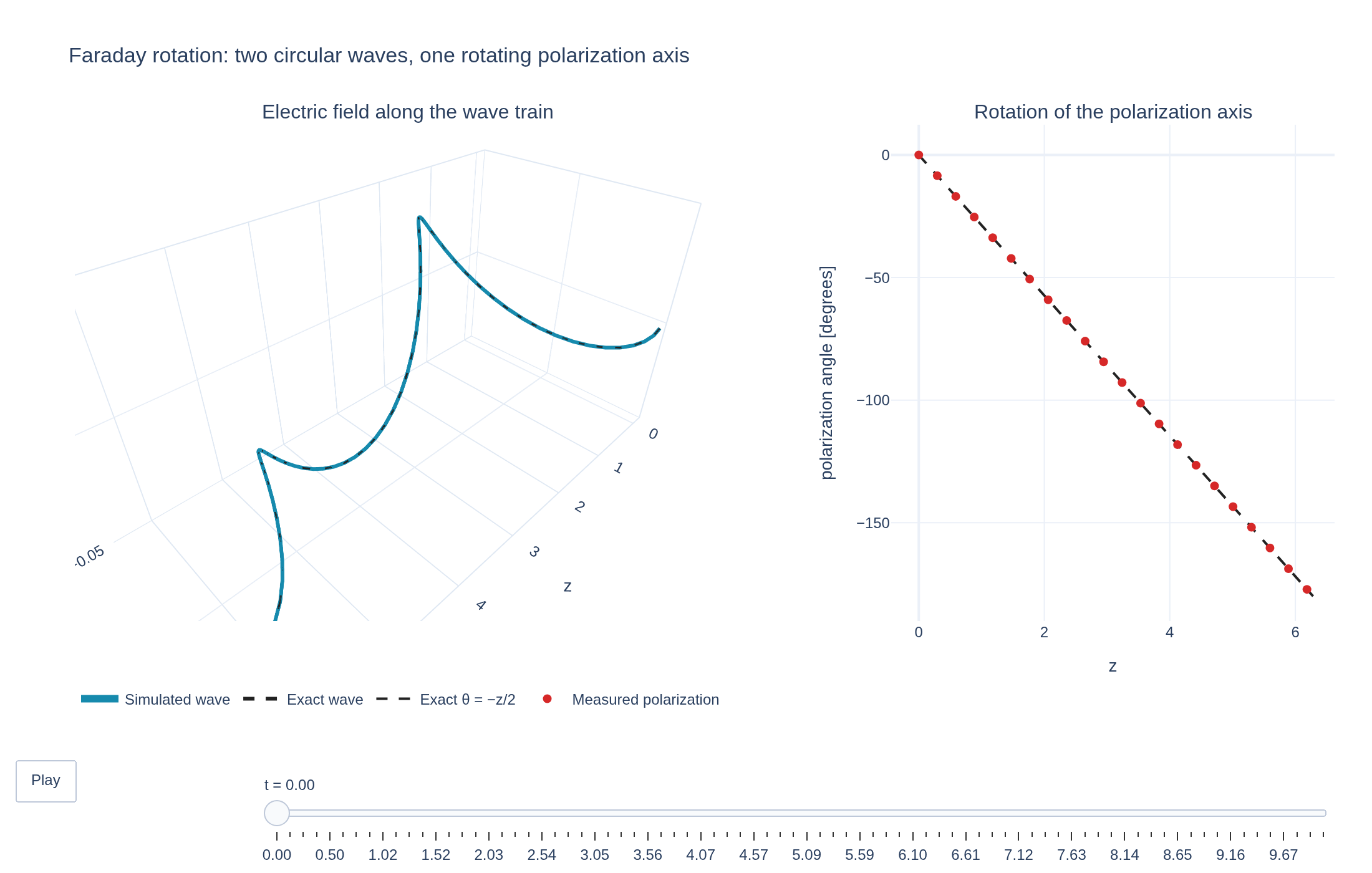
Loading interactive figure…
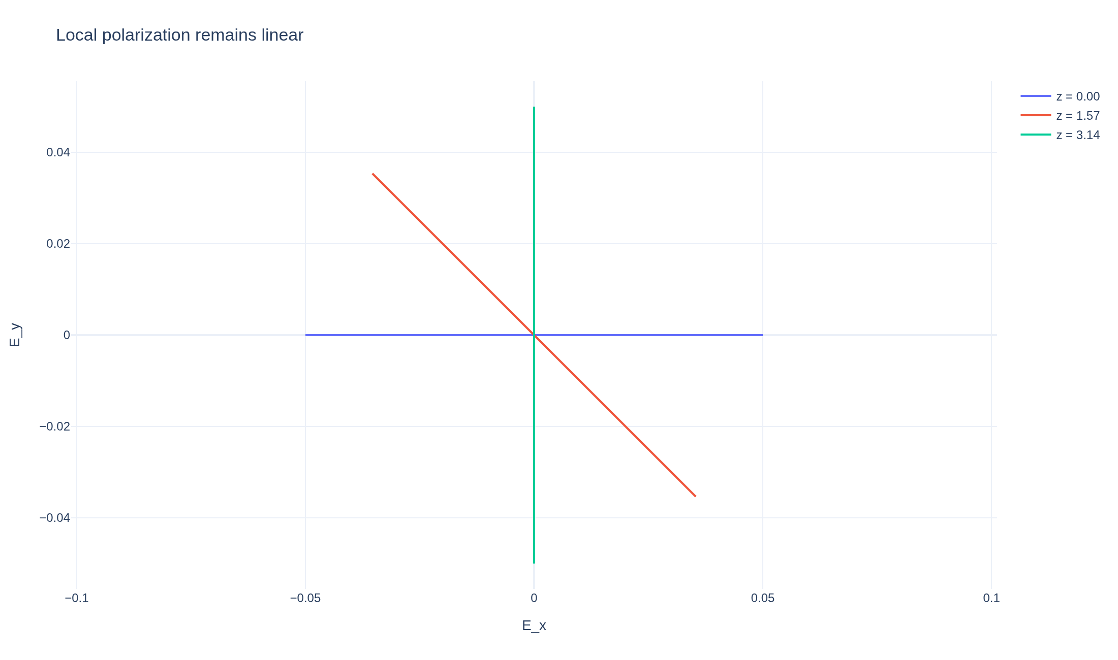
Physical problem
Two circular waves rotate a linear polarization
PDEs solved by model:
Cold-plasma current:
Faraday's law:
Ampère's law:
where denotes an inhomogeneous background.
Simulation geometry
Domain used in this run
The actual Cuboid geometry reconstructed from this run's metadata. Switch between the 3D view and physical-coordinate slices.
Domain
Cuboid
Mapping
Loading Cuboid…
Parameters
| Parameter | Value | Description |
|---|---|---|
| Loading parameters… | ||
Performance
Profiling
Struphy's built-in scope-profiler instruments every propagator, pusher and solver call — these are the real per-call timings from the run above.
Durations
Gantt (rank 0)
Region statistics
| Region | Count | Avg (s) | Min (s) | Max (s) | Total (s) |
|---|
Complete source
Simulation script
Requires Struphy with compiled kernels and Plotly. Run struphy compile once, then execute python faraday-rotation.py.
"""Faraday rotation as a superposition of two circular cold-plasma eigenmodes.

Choose omega = 2.5, Omega_c = 1 and omega_p**2 = n0 = 3.15, so the two
parallel circular modes have exactly k = 1 and 2. Both fit the periodic box.
Their equal-amplitude sum is linearly polarized at every z, with an axis that
rotates as theta(z) = -z/2 for the signed-current convention used here (epsilon=1).
This initializes an established wave train, not a pulse injected at a boundary.

Reference: https://farside.ph.utexas.edu/teaching/315/Waveshtml/node76.html
Requires the pinned Struphy with compiled kernels (`struphy compile`).
"""

import numpy as np

from struphy import DerhamOptions, EnvironmentOptions, Simulation, Time, domains, equils, grids, perturbations
from struphy.models import ColdPlasma
from struphy.linear_algebra.solver import SolverParameters

stem = "faraday-rotation"
length, amplitude, omega, density = 2.0 * np.pi, 0.05, 2.5, 3.15
period = 2.0 * np.pi / omega
model = ColdPlasma(alpha=1.0, epsilon=1.0)
for propagator in (model.propagators.maxwell, model.propagators.ohm, model.propagators.jxb):
    propagator.options = propagator.Options(solver_params=SolverParameters(tol=1e-12))

# With exp(i(kz - omega*t)), E = (1, i*s), j = i*n0*E/(omega+s).
# The corresponding dispersion law is k² = omega² - n0*omega/(omega+s).
for k, helicity in ((1, -1), (2, 1)):
    half = amplitude / 2.0
    for variable, component, mode, value in (
        (model.em_fields.e_field, 0, perturbations.ModesCos, half),
        (model.em_fields.e_field, 1, perturbations.ModesSin, -helicity * half),
        (model.em_fields.b_field, 0, perturbations.ModesSin, helicity * k / omega * half),
        (model.em_fields.b_field, 1, perturbations.ModesCos, k / omega * half),
        (model.electrons.current, 0, perturbations.ModesSin, -density / (omega + helicity) * half),
        (model.electrons.current, 1, perturbations.ModesCos, -helicity * density / (omega + helicity) * half),
    ):
        variable.add_perturbation(mode(ns=(k,), amps=(value,), comp=component, Lz=length, given_in_basis="physical"))

domain = domains.Cuboid(r3=length)
grid = grids.TensorProductGrid(num_elements=(1, 1, 64))
derham_opts = DerhamOptions(degree=(1, 1, 3))
time_opts = Time(dt=period / 250.0, Tend=4.0 * period, split_algo="Strang")
sim = Simulation(
    model=model, name="Faraday rotation in a magnetized plasma",
    description=(
        "Two circularly polarized waves of equal frequency and amplitude travel along the magnetic field. "
        "Their different wavelengths rotate the plane of their combined, linearly polarized electric field: "
        "the Faraday effect. This periodic example starts with the complete wave train, including its current and magnetic field."
        r" With :math:`\omega=2.5`, :math:`B_0=1` and :math:`n_0=3.15`, the wavenumbers are :math:`k_1=1` and :math:`k_2=2`."
        r" The electric field is $$\mathbf{E}_\perp(z,t)=0.05\cos(1.5z-2.5t)(\cos(z/2),-\sin(z/2)),$$"
        r" so the polarization axis rotates by :math:`\theta(z)=-z/2`, modulo :math:`\pi`, in this sign convention."
    ),
    env=EnvironmentOptions(out_folders="struphy_gallery_runs", sim_folder="faraday_rotation"),
    time_opts=time_opts, domain=domain, grid=grid, derham_opts=derham_opts,
    equil=equils.HomogenSlab(B0z=1.0, n0=density),
)


if __name__ == "__main__":
    import plotly.graph_objects as go
    from plotly.subplots import make_subplots
    from _gallery import export_profiling, merge_metadata, save_extra_figure, save_figure

    output = sim.run(profiling_activated=True)
    output.pproc(physical=True)
    field = output.evaluate("em_fields/e_field_xyz").isel(e1=0, e2=0)
    ex, ey = (field.isel(component=i).values for i in (0, 1))
    times, z = field.t.values, field.e3.values * length
    energy = output.evaluate("total_energy")
    if not all(np.isfinite(a).all() for a in (ex, ey, energy.values)) or not np.isclose(times[-1], time_opts.Tend):
        raise RuntimeError("The Faraday run is incomplete or non-finite")
    carrier = amplitude * np.cos(1.5 * z[None, :] - omega * times[:, None])
    exact_x, exact_y = carrier * np.cos(z / 2), -carrier * np.sin(z / 2)
    error = float(np.max(np.hypot(ex - exact_x, ey - exact_y)) / amplitude)
    # Fit the complex phasors over four periods. Stokes Q,U give the polarization
    # axis even at locations/times where the instantaneous electric field vanishes.
    temporal_basis = np.column_stack((np.cos(omega * times), np.sin(omega * times), np.ones_like(times)))
    ax = np.linalg.lstsq(temporal_basis, ex, rcond=None)[0]
    ay = np.linalg.lstsq(temporal_basis, ey, rcond=None)[0]
    phasor_x, phasor_y = ax[0] + 1j * ax[1], ay[0] + 1j * ay[1]
    q = np.abs(phasor_x)**2 - np.abs(phasor_y)**2
    u = 2.0 * np.real(phasor_x * phasor_y.conj())
    angle = 0.5 * np.unwrap(np.arctan2(u, q))
    rotation_rate = float(np.polyfit(z, angle, 1)[0])
    angle_error = float(np.max(np.abs(angle + z / 2)))
    energy_drift = float(np.max(np.abs(energy.values / energy.values[0] - 1.0)))
    if error > 0.03 or angle_error > 0.02 or energy_drift > 1e-6:
        raise RuntimeError(f"Faraday check failed: field={error:.3g}, angle={angle_error:.3g}, energy={energy_drift:.3g}")

    figure = make_subplots(rows=1, cols=2, specs=[[{"type": "scene"}, {"type": "xy"}]],
                           column_widths=[0.6, 0.4], horizontal_spacing=0.12,
                           subplot_titles=("Electric field along the wave train", "Rotation of the polarization axis"))
    figure.add_trace(go.Scatter3d(x=z, y=ex[0], z=ey[0], mode="lines", name="Simulated wave",
                                  line={"color": "#168aad", "width": 6}), row=1, col=1)
    figure.add_trace(go.Scatter3d(x=z, y=exact_x[0], z=exact_y[0], mode="lines", name="Exact wave",
                                  line={"color": "#222", "width": 3, "dash": "dash"}), row=1, col=1)
    figure.add_scatter(x=z, y=-z * 90 / np.pi, name="Exact θ = −z/2", line={"color": "#222", "dash": "dash"}, row=1, col=2)
    figure.add_scatter(x=z[::3], y=np.degrees(angle[::3]), mode="markers", name="Measured polarization",
                       marker={"color": "#d62828", "size": 7}, row=1, col=2)
    picks = np.unique(np.linspace(0, len(times) - 1, 80, dtype=int))
    figure.frames = [go.Frame(name=f"{times[i]:.2f}", traces=[0, 1], data=[
        go.Scatter3d(x=z, y=ex[i], z=ey[i]), go.Scatter3d(x=z, y=exact_x[i], z=exact_y[i]),
    ]) for i in picks]
    figure.update_layout(
        title="Faraday rotation: two circular waves, one rotating polarization axis", template="plotly_white",
        scene={"xaxis_title": "z", "yaxis_title": "E_x", "zaxis_title": "E_y",
               "yaxis": {"range": [-amplitude, amplitude]}, "zaxis": {"range": [-amplitude, amplitude]},
               "aspectmode": "manual", "aspectratio": {"x": 2, "y": 1, "z": 1}},
        margin={"l": 60, "r": 30, "t": 100, "b": 170}, legend={"orientation": "h", "y": -0.12},
        updatemenus=[{"type": "buttons", "showactive": False, "x": 0, "y": -0.28,
                      "buttons": [{"label": "Play", "method": "animate", "args": [None, {"frame": {"duration": 70, "redraw": True}, "transition": {"duration": 0}, "fromcurrent": True}]}]}],
        sliders=[{"x": 0.15, "len": 0.85, "y": -0.25, "currentvalue": {"prefix": "t = "},
                  "steps": [{"method": "animate", "label": f.name, "args": [[f.name], {"mode": "immediate", "frame": {"duration": 0, "redraw": True}, "transition": {"duration": 0}}]} for f in figure.frames]}],
    )
    figure.update_xaxes(title_text="z", row=1, col=2)
    figure.update_yaxes(title_text="polarization angle [degrees]", row=1, col=2)
    save_figure(figure, stem, height=700)
    probes = go.Figure()
    for target in (0.0, length / 4, length / 2):
        j = int(np.argmin(np.abs(z - target)))
        probes.add_scatter(x=ex[:, j], y=ey[:, j], name=f"z = {z[j]:.2f}", mode="lines")
    probes.update_layout(title="Local polarization remains linear", template="plotly_white",
                          xaxis_title="E_x", yaxis_title="E_y", yaxis={"scaleanchor": "x"},
                          margin={"l": 70, "r": 30, "t": 80, "b": 70})
    figures = [save_extra_figure(probes, stem, "polarization", alt="Electric-field hodographs forming lines at three different angles",
                                caption="At each position the electric vector traces a line. Its orientation changes with distance along the magnetic field.")]
    merge_metadata(stem, measuredRotationRate=rotation_rate, exactRotationRate=-0.5,
                   maxRelativeFieldError=error, maxAngleErrorRadians=angle_error, maxEnergyDrift=energy_drift,
                   figures=figures, **export_profiling(sim, stem))
See the post-processing guide for more ways to inspect the result.