Maxwell · Numerical methods
Structure preservation in time integration
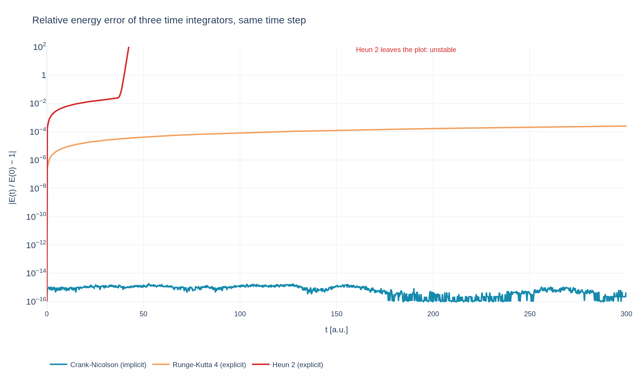
One standing electromagnetic wave, stepped by Crank-Nicolson, RK4 and Heun's method at the same time step. The symplectic implicit scheme keeps the energy error bounded for the whole run, while the explicit schemes do not: RK4 loses energy steadily, and Heun's method is unstable for this operator.

Physical problem
One wave, three time integrators
One standing electromagnetic wave, stepped by Crank-Nicolson, RK4 and Heun's method at the same time step. The symplectic implicit scheme keeps the energy error bounded for the whole run, while the explicit schemes do not: RK4 loses energy steadily, and Heun's method is unstable for this operator.
PDEs solved by model:
Ampère's law (no current):
Faraday's law:
Simulation geometry
Domain used in this run
The actual Cuboid geometry reconstructed from this run's metadata. Switch between the 3D view and physical-coordinate slices.
Domain
Cuboid
Mapping
Loading Cuboid…
Parameters
| Parameter | Value | Description |
|---|---|---|
| Loading parameters… | ||
- Model
- Maxwell
- Domain
- Cuboid (r3=20)
- Grid
- 1 × 1 × 32
- FEEC degree
- 1 × 1 × 3
- Integrator
- Implicit
- Evolution
- 1,200 steps
- Visualization
- Plotly
Performance
Profiling
Struphy's built-in scope-profiler instruments every propagator, pusher and solver call — these are the real per-call timings from the run above.
Durations
Gantt (rank 0)
Region statistics
| Region | Count | Avg (s) | Min (s) | Max (s) | Total (s) |
|---|
Complete source
Simulation script
Requires Struphy with compiled kernels and Plotly. Run struphy compile once, then execute python maxwell-structure-preservation.py.
"""What "structure-preserving" buys you: three time integrators on the same Maxwell wave.

Struphy's FEEC discretization of Maxwell's equations conserves the electromagnetic energy exactly when
the time integrator does — the implicit midpoint rule (Crank-Nicolson) is symplectic, so its energy
error stays bounded for arbitrarily long runs. Explicit Runge-Kutta schemes are not: they damp or
amplify the fields a little at every step, and that error accumulates in one direction.

The same standing wave in a periodic box is stepped by all three schemes with the same time step:
Crank-Nicolson, classical RK4 and Heun's second-order method. Their energy errors differ by more than two
hundred orders of magnitude: Crank-Nicolson holds the energy at round-off, RK4 is stable but loses a little
at every step, and Heun's method is unstable for this operator and grows without bound. The stability limit
is set by the largest eigenvalue the grid supports, not by the wave being modelled, so a smooth initial
condition does not save it: round-off seeds the unstable modes and they take over.

Requires Struphy 3.3 with compiled kernels (`struphy compile`).
"""

import numpy as np
import plotly.graph_objects as go

from struphy import DerhamOptions, EnvironmentOptions, Simulation, Time, domains, grids, perturbations
from struphy.models import Maxwell
from struphy.ode.utils import ButcherTableau

length = 20.0
mode_number = 2
amplitude = 0.1
wavenumber = 2.0 * np.pi * mode_number / length
frequency = wavenumber  # omega = c k with c = 1
periods = 30

domain = domains.Cuboid(r3=length)
grid = grids.TensorProductGrid(num_elements=(1, 1, 32))
derham_opts = DerhamOptions(degree=(1, 1, 3))
time_opts = Time(dt=(2.0 * np.pi / frequency) / 40.0, Tend=periods * 2.0 * np.pi / frequency)

# The three schemes, all at the same time step.
schemes = {
    "Crank-Nicolson (implicit)": {"algo": "implicit"},
    "Runge-Kutta 4 (explicit)": {"algo": "explicit", "butcher": ButcherTableau(algo="rk4")},
    "Heun 2 (explicit)": {"algo": "explicit", "butcher": ButcherTableau(algo="heun2")},
}


def build_simulation(label, options, **extra):
    """The same standing wave, stepped by one of the schemes."""
    model = Maxwell()
    model.propagators.maxwell.options = model.propagators.maxwell.Options(**options)
    model.em_fields.e_field.add_perturbation(
        perturbations.ModesSin(ns=(mode_number,), amps=(amplitude,), comp=0, Lz=length, given_in_basis="physical"),
    )
    folder = "maxwell_" + label.split(" ")[0].lower().replace("-", "_")
    return Simulation(
        model=model,
        env=EnvironmentOptions(out_folders="struphy_gallery_runs", sim_folder=folder),
        time_opts=time_opts,
        domain=domain,
        grid=grid,
        derham_opts=derham_opts,
        **extra,
    )


reference_label = "Crank-Nicolson (implicit)"
sim = build_simulation(
    reference_label,
    schemes[reference_label],
    name="Structure preservation in time integration",
    description=(
        "One standing electromagnetic wave, stepped by Crank-Nicolson, RK4 and Heun's method at the same "
        "time step. The symplectic implicit scheme keeps the energy error bounded for the whole run, while "
        "the explicit schemes do not: RK4 loses energy steadily, and Heun's method is unstable for this "
        "operator."
    ),
)


if __name__ == "__main__":
    from _gallery import export_profiling, merge_metadata, save_extra_figure, save_figure

    runs = {}
    for label, options in schemes.items():
        simulation = sim if label == reference_label else build_simulation(label, options)
        runs[label] = simulation.run(profiling_activated=label == reference_label)
        # Every rank post-processes: the field profile below is evaluated from the FEEC output, which
        # under MPI is not materialized on first use.
        runs[label].pproc()

    colors = {
        "Crank-Nicolson (implicit)": "#168aad",
        "Runge-Kutta 4 (explicit)": "#f4a261",
        "Heun 2 (explicit)": "#d62828",
    }
    drifts = {}
    figure = go.Figure()
    for label, run in runs.items():
        total = run.evaluate("total_energy")
        time = total.t.values
        relative_error = np.abs(total.values / total.values[0] - 1.0)
        drifts[label] = float(np.max(relative_error))
        print(f"{label}: largest relative energy error over {periods} periods {drifts[label]:.3e}")
        figure.add_scatter(x=time, y=np.clip(relative_error, 1e-16, None), mode="lines", name=label,
                           line={"color": colors[label], "width": 2.5})
    if not np.isfinite(drifts[reference_label]) or drifts[reference_label] > 1e-8:
        raise RuntimeError(f"The implicit scheme did not conserve the energy: {drifts[reference_label]}")
    figure.update_layout(
        title="Relative energy error of three time integrators, same time step",
        xaxis_title="t [a.u.]", yaxis_title="|E(t) / E(0) − 1|",
        template="plotly_white", autosize=True,
        legend={"orientation": "h", "y": -0.18},
        margin={"l": 80, "r": 30, "t": 80, "b": 100},
    )
    # The unstable run spans two hundred decades; clipping the axis keeps the other two readable.
    figure.update_yaxes(type="log", range=[-16.5, 2.0], exponentformat="power")
    figure.add_annotation(x=0.62, xref="paper", y=1.8, text="Heun 2 leaves the plot: unstable", showarrow=False,
                          font={"color": "#d62828"}, bgcolor="rgba(255,255,255,0.8)")
    save_figure(figure, "maxwell-structure-preservation")

    # What the drift does to the solution: the field profile at the end of the run against the exact one.
    stable = [label for label in runs if drifts[label] < 1.0]
    profile = go.Figure()
    for label in stable:
        run = runs[label]
        field = run.evaluate("em_fields/e_field").isel(component=0, e1=0, e2=0, t=-1)
        z = field.e3.values * length
        profile.add_scatter(x=z, y=field.values, mode="lines", name=label,
                            line={"color": colors[label], "width": 2.5})
    exact_field = runs[reference_label].evaluate("em_fields/e_field").isel(component=0, e1=0, e2=0, t=0)
    z = exact_field.e3.values * length
    end_time = periods * 2.0 * np.pi / frequency
    profile.add_scatter(x=z, y=exact_field.values * np.cos(frequency * end_time), mode="markers",
                        name="exact", marker={"color": "#264653", "size": 5, "symbol": "circle-open"})
    profile.update_layout(
        title=f"Electric field after {periods} wave periods",
        xaxis_title="z [a.u.]", yaxis_title="E₁ (logical component)",
        template="plotly_white", autosize=True,
        legend={"orientation": "h", "y": -0.18},
        margin={"l": 80, "r": 30, "t": 80, "b": 100},
    )
    figures = [
        save_extra_figure(
            profile, "maxwell-structure-preservation", "profile",
            alt="The electric field profile after thirty wave periods for the three time integrators",
            caption=(
                f"The field after {periods} periods, for the schemes that stayed stable. Both still sit on "
                "the exact standing-wave profile, so the energy differences above are not visible here: the "
                "cost of the explicit scheme is a slow, one-directional loss rather than a wrong shape. "
                "Heun's method is left out because its solution has diverged by this time. All runs share "
                "the same FEEC space discretization and the same time step — only the time integrator differs."
            ),
        ),
    ]

    merge_metadata(
        "maxwell-structure-preservation",
        **{
            "energyErrorCrankNicolson": drifts["Crank-Nicolson (implicit)"],
            "energyErrorRK4": drifts["Runge-Kutta 4 (explicit)"],
            "energyErrorHeun2": drifts["Heun 2 (explicit)"],
            "wavePeriods": periods,
        },
        figures=figures,
        **export_profiling(sim, "maxwell-structure-preservation"),
    )
See the post-processing guide for more ways to inspect the result.