Maxwell · Electromagnetism
Electromagnetic pulse on a distorted mesh
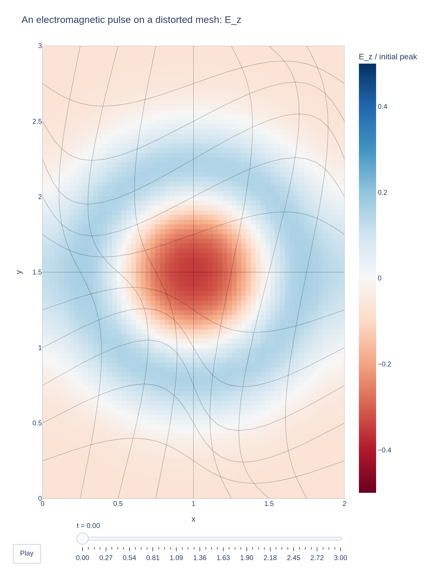
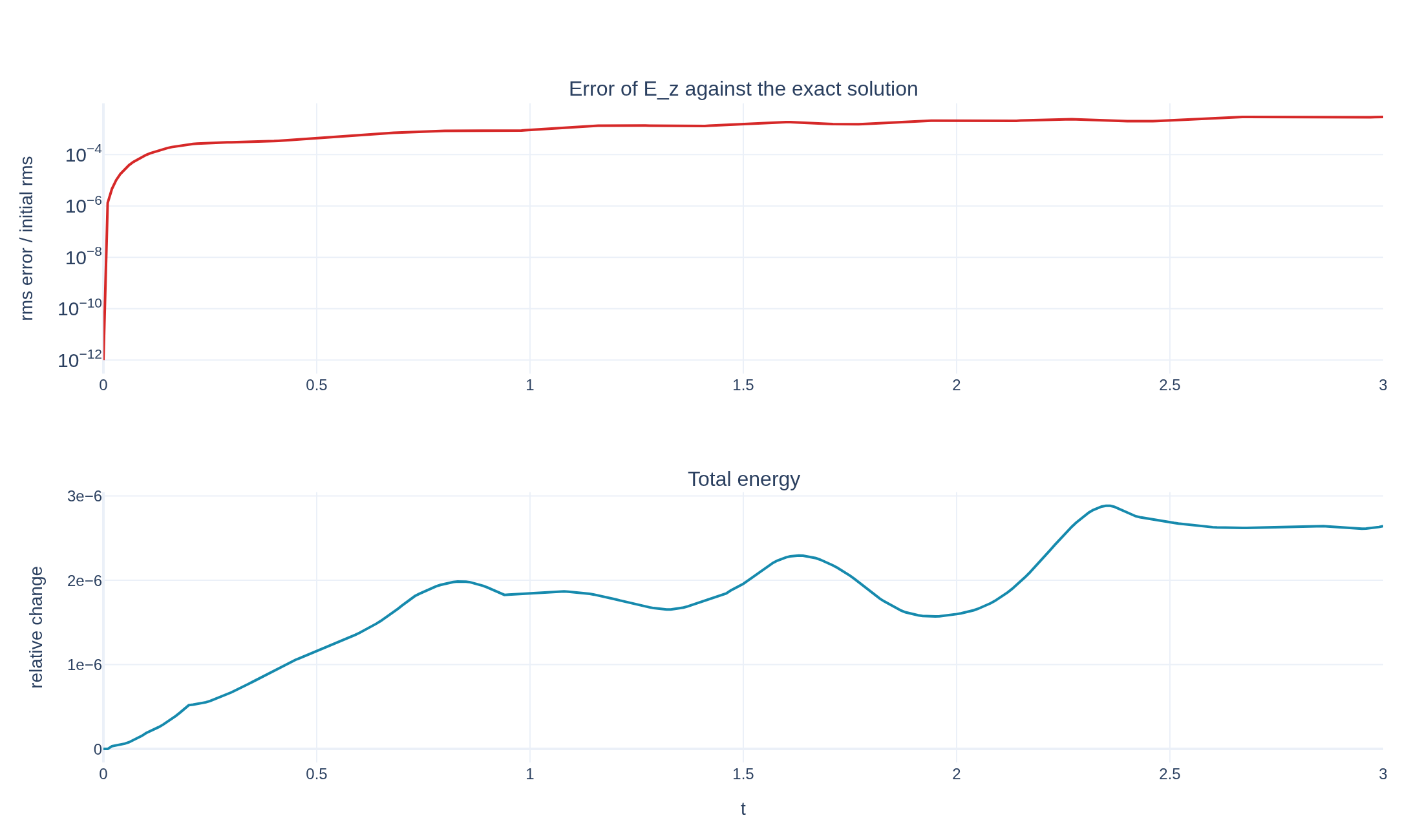
A Gaussian pulse of the electric field spreads as a ring across a periodic box, on a mesh that the Colella mapping has bent. The structure-preserving Maxwell solver keeps the energy constant and follows the exact solution, which is a sum of cosine modes.
Loading interactive figure…
Loading interactive figure…
Physical problem
A pulse on a bent mesh
PDEs solved by model:
Ampère's law (no current):
Faraday's law:
Simulation geometry
Domain used in this run
The actual Colella geometry reconstructed from this run's metadata. Switch between the 3D view and physical-coordinate slices.
Domain
Colella
Mapping
Loading Colella…
Parameters
| Parameter | Value | Description |
|---|---|---|
| Loading parameters… | ||
Performance
Profiling
Struphy's built-in scope-profiler instruments every propagator, pusher and solver call — these are the real per-call timings from the run above.
Durations
Gantt (rank 0)
Region statistics
| Region | Count | Avg (s) | Min (s) | Max (s) | Total (s) |
|---|
Complete source
Simulation script
Requires Struphy with compiled kernels and Plotly. Run struphy compile once, then execute python maxwell-curved-mesh.py.
"""An electromagnetic pulse on a distorted mesh, with Struphy's Maxwell model.

The Colella mapping x = Lx (eta1 + alpha sin(2 pi eta1) sin(2 pi eta2)), y = Ly (eta2 + alpha sin(2 pi eta2) sin(2 pi eta1)) leaves the
boundary of the box [0, Lx] x [0, Ly] where it is but bends the mesh lines inside it. Struphy's finite element spaces are built on the
logical cube and pushed forward with this map, so Maxwell's equations are solved on a curved mesh. Because the physical domain is
still the periodic rectangle, the exact solution is known: a Gaussian pulse of E_z, with B = 0 at first, is a sum of cosine modes,
each oscillating at omega = c |k|, and it can be compared with the numerical field at every point of the distorted mesh. The
energy, which the structure-preserving scheme conserves for any mesh, is followed as well.

Requires Struphy 3.3 with compiled kernels (`struphy compile`).
"""

import numpy as np
import plotly.graph_objects as go

from struphy import DerhamOptions, EnvironmentOptions, Simulation, Time, domains, grids
from struphy.initial.base import GenericPerturbation
from struphy.models import Maxwell

lx, ly = 2.0, 3.0
distortion = 0.1
width = 0.25  # of the Gaussian pulse
max_mode = 6  # cosine modes per direction in the Fourier series of the Gaussian
x0, y0 = 0.5 * lx, 0.5 * ly
time_opts = Time(dt=0.01, Tend=3.0)

# The Gaussian pulse as a cosine series about its centre, E_z = sum c_lm cos(kx (x - x0)) cos(ky (y - y0)) without the mean (l, m) = (0, 0).
modes = [(l, m) for l in range(max_mode + 1) for m in range(max_mode + 1) if (l, m) != (0, 0)]
kx = np.array([2 * np.pi * l / lx for l, _ in modes])
ky = np.array([2 * np.pi * m / ly for _, m in modes])
weights = np.array([(1 if l == 0 else 2) * (1 if m == 0 else 2) for l, m in modes])
coefficients = weights * 2 * np.pi * width**2 / (lx * ly) * np.exp(-0.5 * width**2 * (kx**2 + ky**2))
frequencies = np.hypot(kx, ky)


def exact_field(x, y, t):
    """E_z(x, y, t): every cosine mode oscillates at c |k|, since B is zero and dE/dt is zero at the start."""
    x, y = np.asarray(x)[..., None], np.asarray(y)[..., None]
    return np.sum(coefficients * np.cos(kx * (x - x0)) * np.cos(ky * (y - y0)) * np.cos(frequencies * t), axis=-1)


model = Maxwell()
model.propagators.maxwell.options = model.propagators.maxwell.Options(algo="implicit")
model.em_fields.e_field.add_perturbation(
    GenericPerturbation(lambda x, y, z: exact_field(x, y, 0.0), given_in_basis="physical", comp=2)
)

domain = domains.Colella(Lx=lx, Ly=ly, alpha=distortion, Lz=1.0)
grid = grids.TensorProductGrid(num_elements=(24, 36, 1))
derham_opts = DerhamOptions(degree=(3, 3, 1))

sim = Simulation(
    model=model,
    name="Electromagnetic pulse on a distorted mesh",
    description=(
        "A Gaussian pulse of the electric field spreads as a ring across a periodic box, on a mesh that the Colella "
        "mapping has bent. The structure-preserving Maxwell solver keeps the energy constant and follows the exact "
        "solution, which is a sum of cosine modes."
    ),
    env=EnvironmentOptions(out_folders="struphy_gallery_runs", sim_folder="maxwell_curved_mesh"),
    time_opts=time_opts,
    domain=domain,
    grid=grid,
    derham_opts=derham_opts,
)


if __name__ == "__main__":
    from plotly.subplots import make_subplots
    from scipy.interpolate import griddata

    from _gallery import export_profiling, merge_metadata, save_extra_figure, save_figure

    output = sim.run(profiling_activated=True)
    output.pproc(physical=True)

    e_z = output.evaluate("em_fields/e_field_xyz").isel(component=2, e3=0)  # (t, e1, e2), on the mesh points
    times = e_z.t.values
    mesh_x, mesh_y = e_z.X.values, e_z.Y.values
    numeric = e_z.transpose("t", "e1", "e2").values
    exact = np.array([exact_field(mesh_x, mesh_y, t) for t in times])
    scale = float(np.abs(exact[0]).max())
    error = np.sqrt(np.mean((numeric - exact) ** 2, axis=(1, 2))) / np.sqrt(np.mean(exact[0] ** 2))
    if not np.isfinite(error).all():
        raise RuntimeError("Non-finite field")
    total = output.evaluate("total_energy").values
    energy_drift = float(np.max(np.abs(total / total[0] - 1.0)))
    print(f"Largest rms error of E_z, relative to the initial rms: {error.max():.3e}")
    print(f"Maximum relative drift of the total energy: {energy_drift:.2e}")

    # Resample the values on the distorted mesh onto a regular grid, for the heatmap.
    x_plot, y_plot = np.linspace(0, lx, 64), np.linspace(0, ly, 96)
    xx, yy = np.meshgrid(x_plot, y_plot)
    points = np.column_stack([mesh_x.ravel(), mesh_y.ravel()])

    def resample(values):
        # Rounded, to keep the frames of the page small.
        return np.round(griddata(points, values.ravel(), (xx, yy), method="linear") / scale, 3)

    picks = np.unique(np.linspace(0, len(times) - 1, 45, dtype=int))
    mesh_lines = [
        go.Scatter(x=mesh_x[i, :], y=mesh_y[i, :], mode="lines", line={"color": "rgba(0,0,0,0.35)", "width": 0.7},
                   showlegend=False, hoverinfo="skip")
        for i in range(0, mesh_x.shape[0], 3)
    ] + [
        go.Scatter(x=mesh_x[:, j], y=mesh_y[:, j], mode="lines", line={"color": "rgba(0,0,0,0.35)", "width": 0.7},
                   showlegend=False, hoverinfo="skip")
        for j in range(0, mesh_x.shape[1], 3)
    ]
    frames_numeric = {i: resample(numeric[i]) for i in picks}
    figure = go.Figure(
        data=[go.Heatmap(z=frames_numeric[picks[0]], x=x_plot, y=y_plot, colorscale="RdBu", zmid=0.0, zmin=-0.5, zmax=0.5,
                         colorbar={"title": "E_z / initial peak"})] + mesh_lines,
        frames=[go.Frame(name=f"{times[i]:.2f}", data=[go.Heatmap(z=frames_numeric[i], x=x_plot, y=y_plot, colorscale="RdBu",
                                                                 zmid=0.0, zmin=-0.5, zmax=0.5)], traces=[0])
                for i in picks],
    )
    figure.update_layout(
        title="An electromagnetic pulse on a distorted mesh: E_z", template="plotly_white", autosize=True,
        xaxis_title="x", yaxis_title="y", margin={"l": 70, "r": 30, "t": 80, "b": 130},
        updatemenus=[{"type": "buttons", "showactive": False, "x": 0, "y": -0.1,
                      "buttons": [{"label": "Play", "method": "animate", "args": [None, {"frame": {"duration": 60, "redraw": True}, "transition": {"duration": 0}, "fromcurrent": True}]}]}],
        sliders=[{"active": 0, "x": 0.12, "len": 0.88, "y": -0.02, "currentvalue": {"prefix": "t = "},
                  "steps": [{"args": [[frame.name], {"frame": {"duration": 0, "redraw": True}, "transition": {"duration": 0}, "mode": "immediate"}], "label": frame.name, "method": "animate"} for frame in figure.frames]}],
    )
    figure.update_xaxes(range=[0, lx], constrain="domain")
    figure.update_yaxes(range=[0, ly], scaleanchor="x")
    save_figure(figure, "maxwell-curved-mesh", width=750, height=1000, static_z=resample(numeric[len(times) // 5]))

    diagnostics = make_subplots(rows=2, cols=1, vertical_spacing=0.18,
                                subplot_titles=("Error of E_z against the exact solution", "Total energy"))
    diagnostics.add_scatter(x=times, y=np.maximum(error, 1e-12), mode="lines", showlegend=False,
                            line={"color": "#d62828", "width": 2}, row=1, col=1)
    diagnostics.add_scatter(x=times, y=total / total[0] - 1.0, mode="lines", showlegend=False,
                            line={"color": "#168aad", "width": 2}, row=2, col=1)
    diagnostics.update_layout(template="plotly_white", autosize=True, margin={"l": 80, "r": 30, "t": 80, "b": 60})
    diagnostics.update_yaxes(title_text="rms error / initial rms", type="log", row=1, col=1)
    diagnostics.update_yaxes(title_text="relative change", exponentformat="e", row=2, col=1)
    diagnostics.update_xaxes(title_text="t", row=2, col=1)
    figures = [
        save_extra_figure(
            diagnostics, "maxwell-curved-mesh", "diagnostics",
            alt="Error of the electric field against the exact solution and change of the total energy over time",
            caption=(
                f"Top: the root-mean-square difference between the computed E_z and the exact solution at the points of the distorted mesh, "
                f"relative to the rms of the initial pulse; its largest value is {error.max():.1e}. Bottom: the change of the total "
                f"energy, at most {energy_drift:.1e} in relative terms: the scheme conserves it whatever the shape of the mesh."
            ),
        ),
    ]

    merge_metadata(
        "maxwell-curved-mesh",
        distortion=distortion,
        maxRelativeError=float(error.max()),
        maxEnergyDrift=energy_drift,
        figures=figures,
        **export_profiling(sim, "maxwell-curved-mesh"),
    )
See the post-processing guide for more ways to inspect the result.