Maxwell · Electromagnetic waves
Maxwell light-wave dispersion
Excite a broadband electric field and recover the vacuum dispersion relation ω = ck with Struphy’s FEEC Maxwell solver. The two transverse electric components start with coefficient-noise amplitude , while . On the periodic interval , the allowed wavenumbers are
Loading interactive figure…
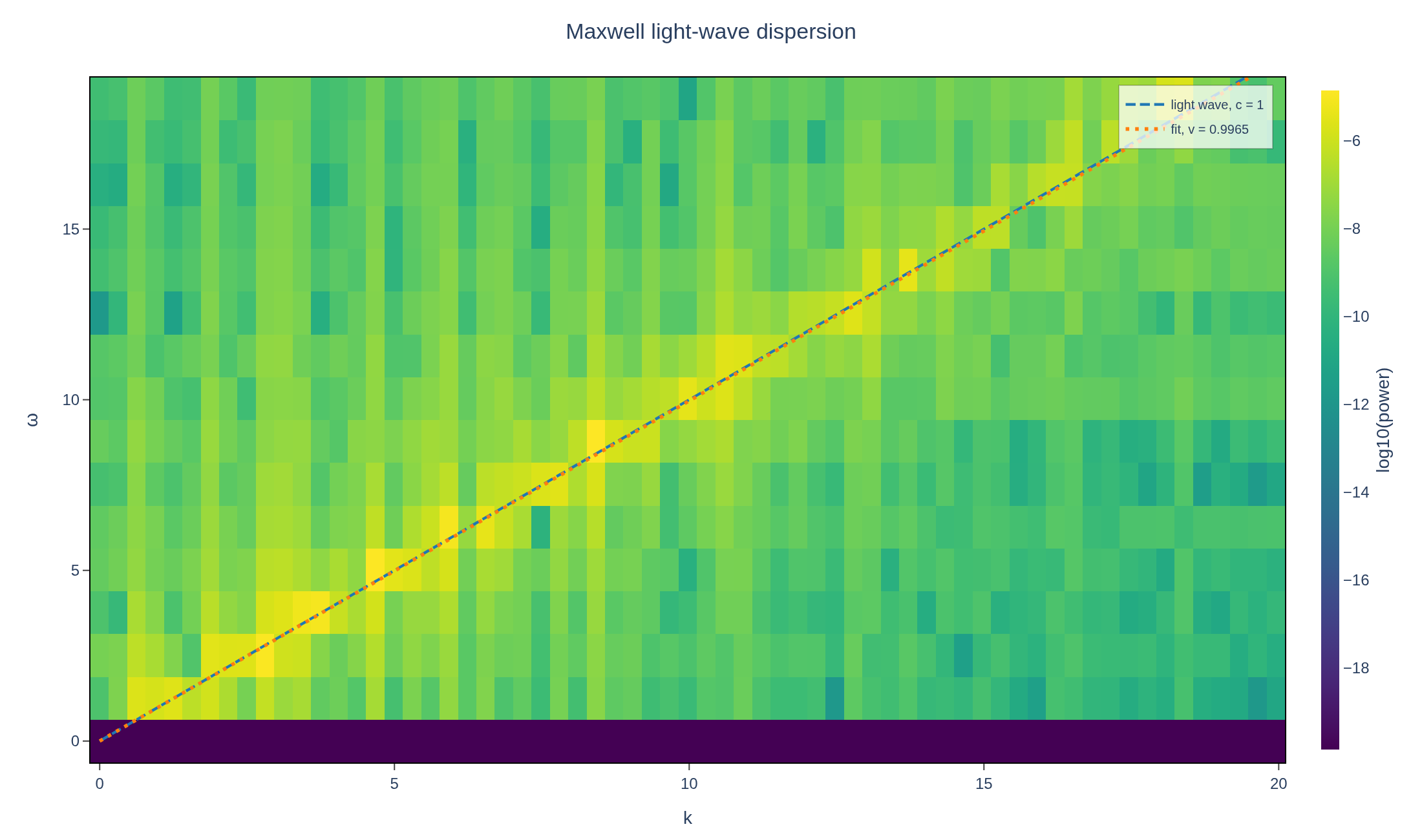
Loading interactive figure…
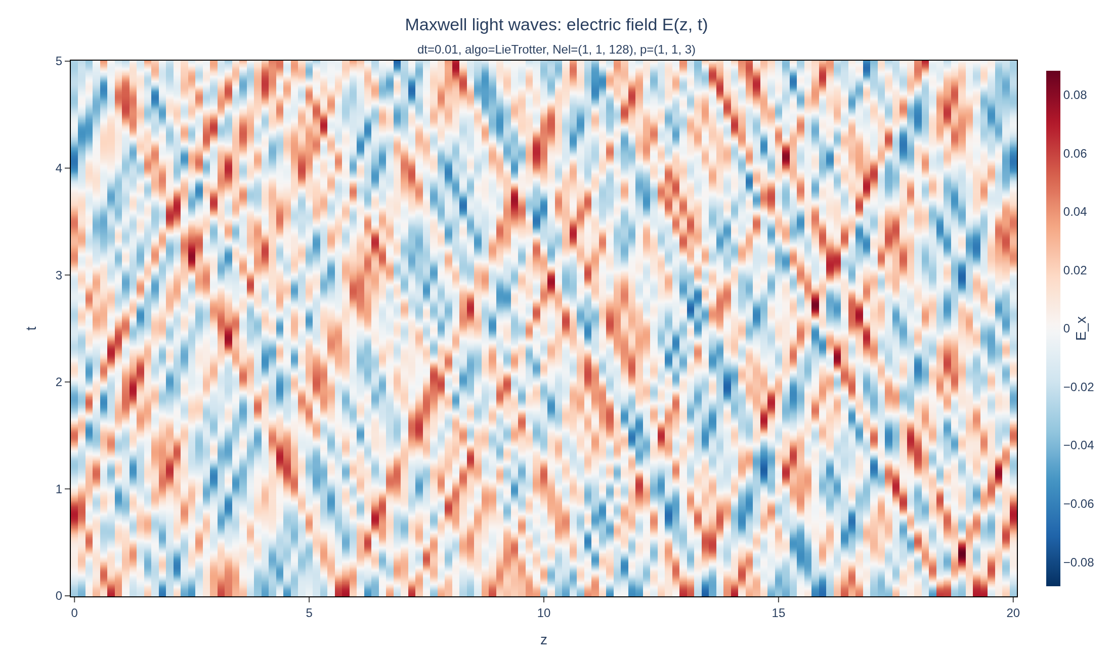
Physical problem
A broadband vacuum light wave
PDEs solved by model:
Ampère's law (no current):
Faraday's law:
Simulation geometry
Domain used in this run
The actual Cuboid geometry reconstructed from this run's metadata. Switch between the 3D view and physical-coordinate slices.
Domain
Cuboid
Mapping
Loading Cuboid…
Parameters
| Parameter | Value | Description |
|---|---|---|
| Loading parameters… | ||
Performance
Profiling
Struphy's built-in scope-profiler instruments every propagator, pusher and solver call — these are the real per-call timings from the run above.
Durations
Gantt (rank 0)
Region statistics
| Region | Count | Avg (s) | Min (s) | Max (s) | Total (s) |
|---|
Complete source
Simulation script
Run it locally
1. Install and compile
Use Python 3.10 or newer with Struphy's system prerequisites installed. Run these commands in your Python environment:
pip install "struphy[pproc]>=3.4.0"
pip install "plasma-plots[plotly]>=0.1.1"
struphy compile
PNG exports need Chrome or Chromium. If Chrome is not installed, run kaleido_get_chrome.
2. Run the script
Download the .py file above, open a terminal in its directory, then run:
python maxwell-wave.pyFigures are saved in the current directory. Add --show to display them before saving.
"""Verify light-wave dispersion with Struphy's Maxwell model.

This compact gallery example follows Struphy's maintained Maxwell verification
test. It excites a broadband electric field, evolves Maxwell's equations with
FEEC, and plots the numerical dispersion relation against omega = c k.

Install dependencies and compile the kernels (Python 3.10 or newer):

    pip install "struphy[pproc]>=3.4.0"
    pip install "plasma-plots[plotly]>=0.1.1"
    struphy compile

PNG exports require Chrome or Chromium. If Chrome is not installed, run:

    kaleido_get_chrome

Save this file and run it from the directory where you want the output:

    python maxwell-wave.py

Figures are saved in the current directory; add --show to display them before saving.
"""

import argparse

import numpy as np

from struphy import (
    DerhamOptions,
    EnvironmentOptions,
    Simulation,
    Time,
    domains,
    grids,
    perturbations,
)
from struphy.models import Maxwell
from plasma_plots import save_figure


def create_simulation() -> Simulation:
    # Model and structure-preserving Maxwell propagator.
    model = Maxwell()
    model.propagators.maxwell.options = model.propagators.maxwell.Options(
        algo="implicit",
    )

    # A periodic one-dimensional domain embedded in 3D.
    domain = domains.Cuboid(r3=20.0)
    grid = grids.TensorProductGrid(num_elements=(1, 1, 128))
    derham_opts = DerhamOptions(degree=(1, 1, 3))
    time_opts = Time(dt=0.01, Tend=5.0)

    # Broadband noise excites several light-wave modes at once.
    model.em_fields.e_field.add_perturbation(
        perturbations.Noise(amp=0.1, comp=0, seed=123),
    )
    model.em_fields.e_field.add_perturbation(
        perturbations.Noise(amp=0.1, comp=1, seed=123),
    )

    env = EnvironmentOptions(
        out_folders="struphy_gallery_runs",
        sim_folder="maxwell_light_wave",
    )
    sim = Simulation(
        model=model,
        name="Maxwell light-wave dispersion",
        description=(
            "Excite a broadband electric field and recover the vacuum dispersion "
            "relation ω = ck with Struphy’s FEEC Maxwell solver."
            r" The two transverse electric components start with coefficient-noise amplitude :math:`A=0.1`, while :math:`\mathbf{B}(z,0)=0`."
            r" On the periodic interval :math:`L_z=20`, the allowed wavenumbers are $$k_n=\frac{2\pi n}{20},\qquad n\in\mathbb{Z}.$$"
        ),
        env=env,
        time_opts=time_opts,
        domain=domain,
        grid=grid,
        derham_opts=derham_opts,
    )
    return sim


def pproc(sim: Simulation, show: bool = False):
    """Measure the speed of light from the (k, omega) spectrum, and save (and show) the figures."""
    from plasma_plots.analysis import power_spectrum

    output = sim.output
    length = sim.domain.params["r3"] - sim.domain.params["l3"]

    # E_x along z over time, at the grid points of the cells and the periodic endpoint, in physical z.
    cells = output.grid.num_elements[2]
    e_x = output.evaluate(
        "em_fields/e_field", eta1=0.0, eta2=0.0, eta3=np.linspace(0.0, 1.0, cells + 1), representation="1"
    ).isel(component=0)
    e_x = e_x.assign_coords(z=("eta3", e_x.eta3.values * length)).swap_dims(eta3="z")

    # The branch of the (k, omega) power spectrum: its peaks count above half the peak amplitude of their
    # k, i.e. a quarter of its peak power.
    spectrum = power_spectrum(e_x, dim="z")
    branch = spectrum.plasma.analysis.fit_branches(n_branches=1, noise_level=0.5**2, order=10)[0]
    print(f"Measured phase velocity: {branch.velocity:.5f} (exact: 1.0)")

    dispersion = spectrum.plasma.plot.dispersion(
        kmin=0,
        branches={"light wave, c = 1": lambda k: k},
        fits=[branch],
        dynamic_range=15,
        omega_max=float(spectrum.k.max()),
        title="Maxwell light-wave dispersion",
        backend="plotly",
    )
    # Waves travelling in both directions leave diagonal stripes, whose slope is the wave speed.
    space_time = e_x.plasma.plot.slice(
        x="z",
        y="t",
        symmetric=True,
        cmap="RdBu_r",
        title="Maxwell light waves: electric field E(z, t)",
        colorbar_label="E_x",
        backend="plotly",
    )
    save_figure(dispersion, "maxwell-wave", show=show)
    save_figure(space_time, "maxwell-wave-space-time", show=show)


if __name__ == "__main__":
    argparser = argparse.ArgumentParser(description="Run the maxwell wave example.")
    argparser.add_argument(
        "--pproc-only",
        action="store_true",
        help="Run post-processing on an existing simulation instead of running a new one.",
    )
    argparser.add_argument("--show", action="store_true", help="Show the figures before saving them.")
    args = argparser.parse_args()

    simulation = create_simulation()
    if not args.pproc_only:
        simulation.run()
    pproc(simulation, show=args.show)
See the post-processing guide for more ways to inspect the result.