ShearAlfven · MHD waves
Standing shear-Alfvén wave
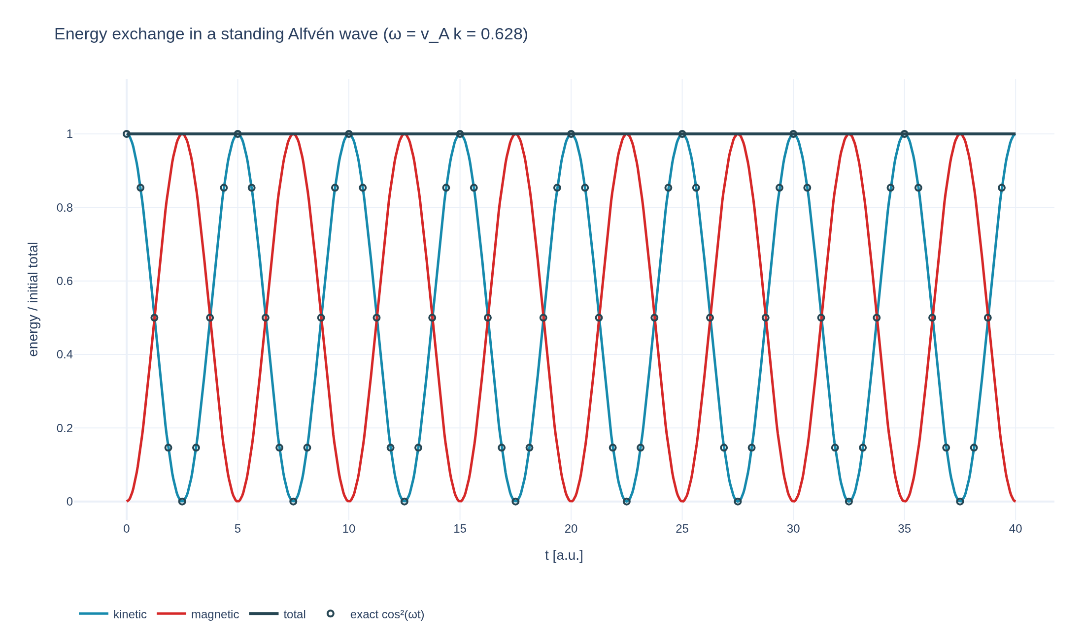
A single transverse velocity mode splits into two counter-propagating Alfvén waves, i.e. a standing wave. Its energy oscillates between the kinetic and the magnetic channel at twice the wave frequency, while the structure-preserving discretization keeps the sum constant.

Physical problem
One mode, two counter-propagating waves
A single transverse velocity mode splits into two counter-propagating Alfvén waves, i.e. a standing wave. Its energy oscillates between the kinetic and the magnetic channel at twice the wave frequency, while the structure-preserving discretization keeps the sum constant.
PDEs solved by model:
Momentum:
Induction:
Simulation geometry
Domain used in this run
The actual Cuboid geometry reconstructed from this run's metadata. Switch between the 3D view and physical-coordinate slices.
Domain
Cuboid
Mapping
Loading Cuboid…
Parameters
| Parameter | Value | Description |
|---|---|---|
| Loading parameters… | ||
- Model
- ShearAlfven
- Domain
- Cuboid (r3=20)
- Grid
- 1 × 1 × 32
- FEEC degree
- 1 × 1 × 3
- Integrator
- Implicit
- Evolution
- 800 steps
- Visualization
- Plotly
Performance
Profiling
Struphy's built-in scope-profiler instruments every propagator, pusher and solver call — these are the real per-call timings from the run above.
Durations
Gantt (rank 0)
Region statistics
| Region | Count | Avg (s) | Min (s) | Max (s) | Total (s) |
|---|
Complete source
Simulation script
Requires Struphy with compiled kernels and Plotly. Run struphy compile once, then execute python alfven-standing-wave.py.
"""A standing shear-Alfvén wave, and the energy it passes back and forth, with Struphy's ShearAlfven model.

A single transverse velocity mode u_x = U sin(k z) in a uniform plasma at rest splits into two Alfvén
waves running in opposite directions. Their sum is a standing wave: the velocity nodes stay where they
are while the whole profile breathes. The energy moves between the two channels, kinetic when the fluid
moves fastest and magnetic a quarter period later when the field lines are bent the most,

    E_kin(t) = E_0 cos^2(omega t),   E_mag(t) = E_0 sin^2(omega t),   omega = v_A k,

so each channel oscillates at twice the wave frequency while their sum stays constant. Struphy's
propagator is a Crank-Nicolson step, which conserves that sum up to the tolerance of the linear solver.

Requires Struphy 3.3 with compiled kernels (`struphy compile`).
"""

import numpy as np
import plotly.graph_objects as go

from struphy import DerhamOptions, EnvironmentOptions, Simulation, Time, domains, equils, grids, perturbations
from struphy.models import ShearAlfven

# A uniform background with B0 along z and n0 = 1, so the Alfvén speed is 1.
B0z, n0, beta = 1.0, 1.0, 0.1
length = 20.0
mode_number = 2  # wavelengths in the box
amplitude = 0.01

alfven_speed = B0z / np.sqrt(n0)
wavenumber = 2.0 * np.pi * mode_number / length
frequency = alfven_speed * wavenumber
period = 2.0 * np.pi / frequency

model = ShearAlfven()

# One mode, transverse to B0: sin(2 pi n z / L) in the velocity, nothing in the magnetic field.
model.mhd.velocity.add_perturbation(
    perturbations.ModesSin(ns=(mode_number,), amps=(amplitude,), comp=0, Lz=length, given_in_basis="physical"),
)

domain = domains.Cuboid(r3=length)
grid = grids.TensorProductGrid(num_elements=(1, 1, 32))
derham_opts = DerhamOptions(degree=(1, 1, 3))
equil = equils.HomogenSlab(B0x=0.0, B0y=0.0, B0z=B0z, n0=n0, beta=beta)
time_opts = Time(dt=period / 200.0, Tend=4.0 * period)

env = EnvironmentOptions(out_folders="struphy_gallery_runs", sim_folder="alfven_standing_wave")
sim = Simulation(
    model=model,
    name="Standing shear-Alfvén wave",
    description=(
        "A single transverse velocity mode splits into two counter-propagating Alfvén waves, i.e. a standing "
        "wave. Its energy oscillates between the kinetic and the magnetic channel at twice the wave frequency, "
        "while the structure-preserving discretization keeps the sum constant."
    ),
    env=env,
    time_opts=time_opts,
    domain=domain,
    equil=equil,
    grid=grid,
    derham_opts=derham_opts,
)


if __name__ == "__main__":
    from _gallery import export_profiling, merge_metadata, save_extra_figure, save_figure, space_time_figure

    output = sim.run(profiling_activated=True)
    output.pproc(physical=True)

    kinetic = output.evaluate("en_U")
    magnetic = output.evaluate("en_B")
    total = output.evaluate("en_tot")
    time = total.t.values
    total_values = total.values
    energy_scale = float(total_values[0])
    relative_drift = float(np.max(np.abs(total_values / energy_scale - 1.0)))
    print(f"Maximum relative drift of the total energy: {relative_drift:.2e}")

    # The exchange period is half the wave period; measure it from the kinetic-energy maxima.
    kinetic_values = kinetic.values
    peaks = np.flatnonzero(
        (kinetic_values[1:-1] > kinetic_values[:-2]) & (kinetic_values[1:-1] >= kinetic_values[2:])
    ) + 1
    if peaks.size < 3:
        raise RuntimeError("Too few kinetic-energy maxima to measure the exchange period")
    measured_period = float(np.mean(np.diff(time[peaks])))
    period_error = abs(measured_period / (0.5 * period) - 1.0)
    print(f"Measured exchange period: {measured_period:.4f} (exact: {0.5 * period:.4f}, error {period_error:.2%})")

    figure = go.Figure()
    figure.add_scatter(x=time, y=kinetic_values / energy_scale, mode="lines", name="kinetic",
                       line={"color": "#168aad", "width": 2.5})
    figure.add_scatter(x=time, y=magnetic.values / energy_scale, mode="lines", name="magnetic",
                       line={"color": "#d62828", "width": 2.5})
    figure.add_scatter(x=time, y=total_values / energy_scale, mode="lines", name="total",
                       line={"color": "#264653", "width": 3})
    # The exact curve lies on top of the measured one, so show it as sparse markers to keep both readable.
    sampled = np.arange(time[0], time[-1], period / 16.0)
    figure.add_scatter(x=sampled, y=np.cos(frequency * sampled) ** 2, mode="markers", name="exact cos²(ωt)",
                       marker={"color": "#264653", "size": 6, "symbol": "circle-open", "line": {"width": 2}})
    figure.update_layout(
        title=f"Energy exchange in a standing Alfvén wave (ω = v_A k = {frequency:.3f})",
        xaxis_title="t [a.u.]", yaxis_title="energy / initial total",
        template="plotly_white", autosize=True,
        legend={"orientation": "h", "y": -0.18},
        margin={"l": 75, "r": 30, "t": 80, "b": 100},
    )
    figure.update_yaxes(range=[-0.05, 1.15])
    save_figure(figure, "alfven-standing-wave")

    # The velocity along z over time: a standing wave keeps its nodes, so the stripes are vertical,
    # unlike the diagonal stripes of the travelling waves in `shear-alfven-wave`.
    velocity = output.evaluate("mhd/velocity").isel(component=0, e1=0, e2=0)
    space_time = space_time_figure(
        velocity,
        space="e3",
        x_values=velocity.e3.values * length,
        xaxis_title="z [a.u.]",
        title="Standing Alfvén wave: transverse velocity u(z, t)",
        colorbar_title="u₁ (logical component)",
    )
    figures = [
        save_extra_figure(
            space_time, "alfven-standing-wave", "space-time",
            alt="Space-time map of the transverse velocity of a standing Alfvén wave, with fixed nodes",
            caption=(
                "The transverse velocity along z, over time. The nodes stay at the same z while the profile "
                "changes sign every half period: the signature of a standing wave, in contrast with the "
                "criss-crossing diagonal stripes of the travelling waves in the broadband example. The "
                f"relative drift of the total energy over {4 * period:.0f} time units stays below "
                f"{relative_drift:.1e}."
            ),
        ),
    ]

    merge_metadata(
        "alfven-standing-wave",
        measuredExchangePeriod=measured_period,
        exactExchangePeriod=0.5 * period,
        exchangePeriodError=period_error,
        relativeEnergyDrift=relative_drift,
        figures=figures,
        **export_profiling(sim, "alfven-standing-wave"),
    )
See the post-processing guide for more ways to inspect the result.