ViscousEulerSPH · Viscous particle flow
SPH velocity diffusion
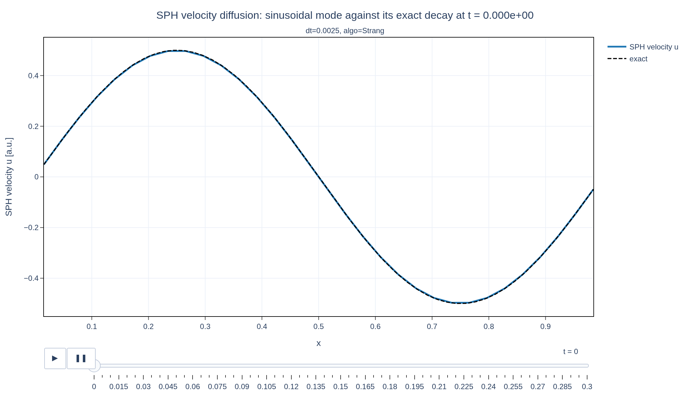
A sinusoidal velocity field diffuses on a periodic interval. The binned SPH current is compared with the exact viscous decay of the mode.
Physical problem
A velocity wave smoothed by viscosity
A sinusoidal velocity field diffuses on a periodic interval. The binned SPH current is compared with the exact viscous decay of the mode.
PDEs solved by model:
Continuity:
Momentum:
Entropy:
where denotes the entropy per unit mass and is the viscous stress tensor.
The viscous stress tensor for a Newtonian fluid is given by:
where is the dynamic (shear) viscosity and is the identity tensor.
The internal energy per unit mass can be defined in two ways:
Simulation geometry
Domain used in this run
The actual Cuboid geometry reconstructed from this run's metadata. Switch between the 3D view and physical-coordinate slices.
Domain
Cuboid
Mapping
Loading Cuboid…
Parameters
| Parameter | Value | Description |
|---|---|---|
| Loading parameters… | ||
- Model
- ViscousEulerSPH
- Domain
- Cuboid
- Integrator
- Forward euler
- Evolution
- 120 steps
- Visualization
- Plotly
Performance
Profiling
Struphy's built-in scope-profiler instruments every propagator, pusher and solver call — these are the real per-call timings from the run above.
Durations
Gantt (rank 0)
Region statistics
| Region | Count | Avg (s) | Min (s) | Max (s) | Total (s) |
|---|
Complete source
Simulation script
Requires Struphy with compiled kernels and Plotly. Run struphy compile once, then execute python sph-velocity-diffusion.py.
"""Viscous decay of a velocity mode with smoothed-particle hydrodynamics.

The pressure-free `ViscousEulerSPH` model starts with a sinusoidal longitudinal
velocity, u(x, 0) = A sin(2 pi x / L), on a periodic interval. Viscosity alone
then damps that mode at 4 mu k^2 / 3, with k = 2 pi / L. The binned SPH current
makes a small, fast verification case with an analytic answer.

Requires Struphy 3.3 with compiled kernels (`struphy compile`).
"""

import numpy as np
import plotly.graph_objects as go

from struphy import (
    BinningPlot,
    BoundaryParameters,
    EnvironmentOptions,
    LoadingParameters,
    SavingParameters,
    Simulation,
    SortingParameters,
    Time,
    WeightsParameters,
    domains,
    equils,
    perturbations,
)
from struphy.models import ViscousEulerSPH
from struphy.ode.utils import ButcherTableau

length = 1.0
viscosity = 0.05
initial_amplitude = 0.5
boxes = 16
markers_per_box = 64
bins = 32
wavenumber = 2 * np.pi / length
exact_decay_rate = viscosity * 4 / 3 * wavenumber**2

# With pressure disabled, this is the particle discretisation of velocity diffusion.
model = ViscousEulerSPH(with_B0=False, with_p=False, with_viscosity=True)
model.propagators.push_eta.options = model.propagators.push_eta.Options(
    butcher=ButcherTableau(algo="forward_euler")
)
model.propagators.push_viscous.options = model.propagators.push_viscous.Options(
    kernel_type="gaussian_1d", mu=viscosity
)

domain = domains.Cuboid(r1=length)
model.euler_fluid.set_markers(
    loading_params=LoadingParameters(ppb=markers_per_box, loading="tesselation"),
    weights_params=WeightsParameters(),
    boundary_params=BoundaryParameters(),
    sorting_params=SortingParameters(boxes_per_dim=(boxes, 1, 1), dims_mask=(True, False, False)),
    saving_params=SavingParameters(
        binning_plots=(
            BinningPlot(slice="e1", n_bins=(bins,), ranges=(0.0, 1.0), output_quantity="current_1"),
        ),
    ),
)
model.euler_fluid.var.add_background(equils.ConstantVelocity())
model.euler_fluid.var.add_perturbation(
    del_u1=perturbations.ModesSin(ls=(1,), amps=(initial_amplitude,))
)

sim = Simulation(
    model=model,
    name="SPH velocity diffusion",
    description=(
        "A sinusoidal velocity field diffuses on a periodic interval. The binned SPH current "
        "is compared with the exact viscous decay of the mode."
    ),
    env=EnvironmentOptions(out_folders="struphy_gallery_runs", sim_folder="sph_velocity_diffusion"),
    time_opts=Time(dt=0.0025, Tend=0.3, split_algo="Strang"),
    domain=domain,
    grid=None,
    derham_opts=None,
)


if __name__ == "__main__":
    from _gallery import export_profiling, is_root, merge_metadata, save_figure

    output = sim.run(profiling_activated=True)
    output.pproc()
    velocity = output.evaluate("euler_fluid/e1_current_1/f")
    times = np.asarray(velocity.t.values)
    x = np.asarray(velocity.e1.values) * length
    values = np.asarray(velocity.values)
    if not np.isfinite(values).all():
        raise RuntimeError("Non-finite SPH velocity: refusing to publish the run")

    # A finite bin records the average of a sine wave, rather than its point value.
    bin_average = np.sinc(wavenumber * (length / bins) / (2 * np.pi))
    mode_amplitude = 2 * np.mean(values * np.sin(wavenumber * x), axis=1) / bin_average
    exact_amplitude = initial_amplitude * np.exp(-exact_decay_rate * times)
    measured_decay_rate = float(-np.polyfit(times, np.log(np.abs(mode_amplitude)), 1)[0])
    relative_rate_error = abs(measured_decay_rate - exact_decay_rate) / exact_decay_rate
    rms_error = float(np.sqrt(np.mean((mode_amplitude - exact_amplitude) ** 2)))
    if is_root():
        print(
            f"decay rate {measured_decay_rate:.4f} (exact {exact_decay_rate:.4f}); "
            f"amplitude RMS error {rms_error:.4g}"
        )

    dense_x = np.linspace(0.0, length, 301)
    picks = np.unique(np.linspace(0, len(times) - 1, min(80, len(times)), dtype=int))

    def profile(index):
        return [
            go.Scatter(
                x=dense_x,
                y=exact_amplitude[index] * np.sin(wavenumber * dense_x),
                mode="lines",
                name="exact",
                line={"color": "#111", "width": 2, "dash": "dash"},
            ),
            go.Scatter(
                x=x,
                y=values[index],
                mode="lines+markers",
                name="SPH",
                line={"color": "#168aad", "width": 2},
                marker={"size": 5},
            ),
        ]

    figure = go.Figure(data=profile(0))
    figure.frames = [go.Frame(name=f"{times[i]:.3f}", data=profile(i)) for i in picks]
    figure.update_layout(
        title="SPH velocity diffusion: sinusoidal mode against its exact decay",
        template="plotly_white",
        xaxis_title="x",
        yaxis_title="u(x, t)",
        yaxis={"range": [-1.1 * initial_amplitude, 1.1 * initial_amplitude]},
        margin={"l": 65, "r": 30, "t": 80, "b": 130},
        legend={"orientation": "h", "y": 1.1},
        updatemenus=[{"type": "buttons", "showactive": False, "x": 0, "y": -0.28, "buttons": [
            {"label": "Play", "method": "animate", "args": [None, {"frame": {"duration": 55, "redraw": False}, "fromcurrent": True}]}
        ]}],
        sliders=[{"x": 0.12, "len": 0.88, "y": -0.18, "currentvalue": {"prefix": "t = "}, "steps": [
            {"args": [[frame.name], {"frame": {"duration": 0, "redraw": False}, "mode": "immediate"}], "label": frame.name, "method": "animate"}
            for frame in figure.frames
        ]}],
    )
    save_figure(figure, "sph-velocity-diffusion")
    merge_metadata(
        "sph-velocity-diffusion",
        viscosity=viscosity,
        exactDecayRate=exact_decay_rate,
        measuredDecayRate=measured_decay_rate,
        relativeRateError=relative_rate_error,
        amplitudeRmsError=rms_error,
        markers=boxes * markers_per_box,
        **export_profiling(sim, "sph-velocity-diffusion"),
    )
See the post-processing guide for more ways to inspect the result.